CCS

Amplitude Modulation (AM)

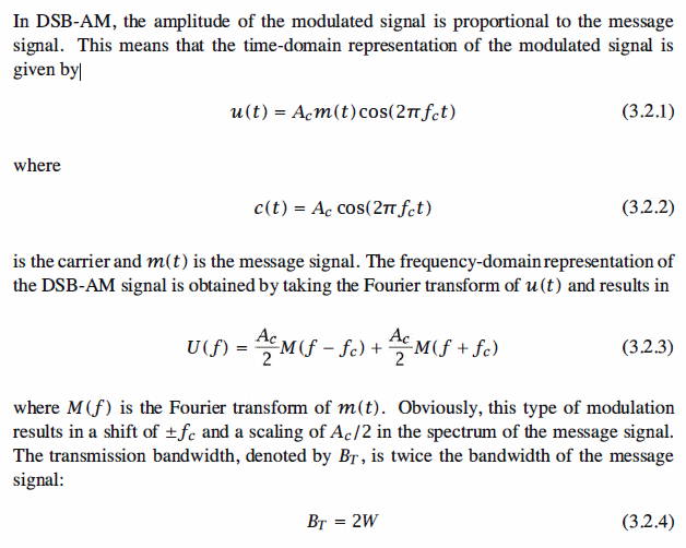
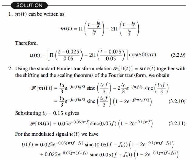
Amplitude modulation (AM), which is frequently referred to as linear modulation, is
the family of modulation schemes in which the amplitude of a sinusoidal carrier is

changed as a function of the modulating signal. This class of modulation schemes
consists of DSB-AM (double-sideband amplitude modulation), conventional amplitude
modulation, SSB-AM (single-sideband amplitude modulation), and VSB-AM
(vestigial-sideband amplitude modulation). The dependence between the modulating
signal and the amplitude of the modulated carrier can be very simple, as, for example,
in the DSB-AM case, or much more complex, as in SSB-AM or VSB-AM. Amplitudemodulation
systems are usually characterized by a relatively low bandwidth requirement
and power inefficiency in comparison to the angle-modulation schemes. The
bandwidth requirement for AM systems varies between W and 2W, where W denotes
the bandwidth of the message signal. For SSB-AM the bandwidth is W, for DSBAM
and conventional AM the bandwidth is 2W, and for VSB-AM the bandwidth
is between W and 2W. These systems are widely used in broadcasting (AM radio
and TV video broadcasting), point-to-point communication (SSB), and multiplexing
applications (for example, transmission of many telephone channels over microwave
links).

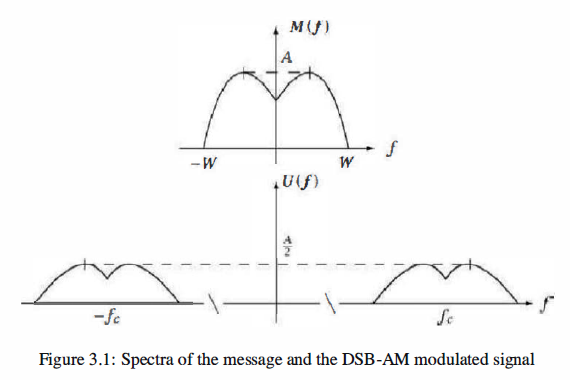
DSB-AM

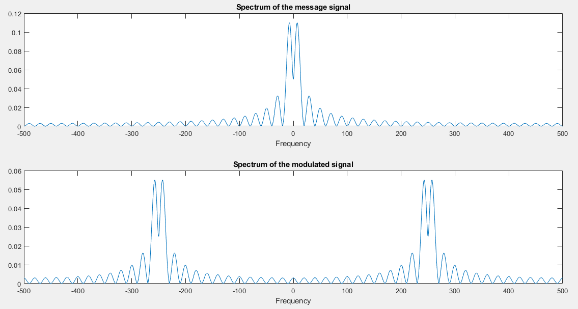
A typical message spectrum and the spectrum of the corresponding DSB-AM modulated
signal are shown in Figure 3 .1.

 

Matlab Coding

 

% MATLAB script for Illustrative Problem 3.1
% Demonstration script for DSB-AM. The message signal is
% +1 for 0 < t < t0/3, -2 for t0/3 < t < 2t0/3, and zero otherwise.

echo on
t0=.15;                                 % signal duration
ts=0.001;                               % sampling interval
fc=250;                                 % carrier frequency
snr=20;                                 % SNR in dB (logarithmic)
fs=1/ts;                                % sampling frequency
df=0.3;                                 % desired freq. resolution
t=[0:ts:t0];                            % time vector
snr_lin=10^(snr/10);                    % linear SNR

% message signal
m=[ones(1,t0/(3*ts)),-2*ones(1,t0/(3*ts)),zeros(1,t0/(3*ts)+1)];
c=cos(2*pi*fc.*t);                      % carrier signal
u=m.*c;                                 % modulated signal
[M,m,df1]=fftseq(m,ts,df);              % Fourier transform
M=M/fs;                                 % scaling
[U,u,df1]=fftseq(u,ts,df);              % Fourier transform
U=U/fs;                                 % scaling
[C,c,df1]=fftseq(c,ts,df);              % Fourier transform
f=[0:df1:df1*(length(m)-1)]-fs/2;       % freq. vector
signal_power=spower(u(1:length(t)));    % power in modulated signal
noise_power=signal_power/snr_lin;       % Compute noise power.
noise_std=sqrt(noise_power);            % Compute noise standard deviation.
noise=noise_std*randn(1,length(u));     % Generate noise.
r=u+noise;                % Add noise to the modulated signal.
[R,r,df1]=fftseq(r,ts,df);       % spectrum of the signal+noise
R=R/fs;                                 % scaling
pause  % Press a key to show the modulated signal power.
signal_power
pause  % Press any key to see a plot of the message.
clf
subplot(2,2,1)
plot(t,m(1:length(t)))
xlabel('Time')
title('The message signal')
pause  % Press any key to see a plot of the carrier.
subplot(2,2,2)
plot(t,c(1:length(t)))
xlabel('Time')
title('The carrier')
pause  % Press any key to see a plot of the modulated signal.
subplot(2,2,3)
plot(t,u(1:length(t)))
xlabel('Time')
title('The modulated signal')
pause   % Press any key to see plots of the magnitude of the message and the
% modulated signal in the frequency domain.
subplot(2,1,1)
plot(f,abs(fftshift(M)))
xlabel('Frequency')
title('Spectrum of the message signal')
subplot(2,1,2)
plot(f,abs(fftshift(U)))
title('Spectrum of the modulated signal')
xlabel('Frequency')
pause  % Press a key to see a noise sample.
subplot(2,1,1)
plot(t,noise(1:length(t)))
title('Noise sample')
xlabel('Time')
pause  % Press a key to see the modulated signal and noise.
subplot(2,1,2)
plot(t,r(1:length(t)))
title('Signal and noise')
xlabel('Time')
pause  % Press a key to see the modulated signal and noise in freq. domain.
subplot(2,1,1)
plot(f,abs(fftshift(U)))
title('Signal spectrum')
xlabel('Frequency')
subplot(2,1,2)
plot(f,abs(fftshift(R)))
title('Signal and noise spectrum')
xlabel('Frequency')

signal_power =

0.8278

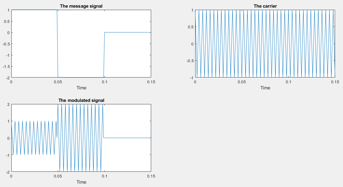
The message, the carrier, and the modulated signal

The modulated signal in the frequency domain(Without Noise)

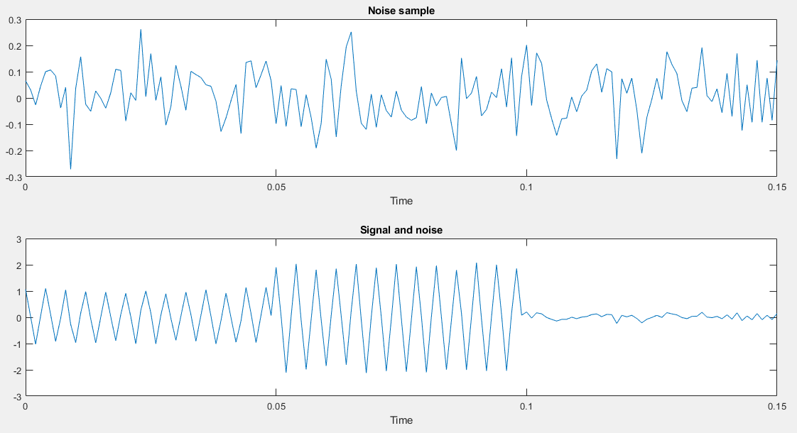
The modulated signal and noise in Time domain

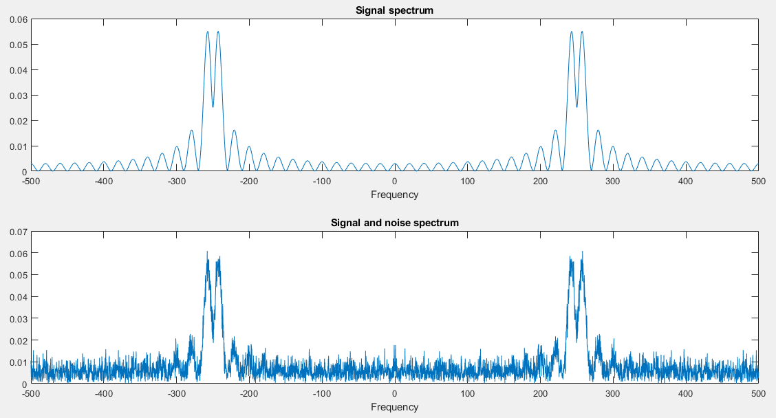
 The modulated signal and noise in freqency domain

Reference,

　　1. <<Contemporary Communication System using MATLAB>> - John G. Proakis