背景:实现一个线性回归模型,根据这个模型去预测一个水库的水位变化而流出的水量。
加载数据集ex5.data1后,数据集分为三部分:
1,训练集(training set)X与y;
2,交叉验证集(cross validation)Xval, yval;
3,测试集(test set): Xtest, ytest。
一:正则化线性回归(Regularized Linear Regression)
1,可视化训练集,如下图所示:
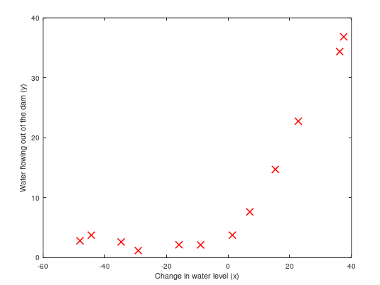
通过可视化数据,接下来我们使用线性回归去拟合这些数据集。
2,正则化线性回归代价函数:
$J( heta)=frac{1}{2m}(sum_{i=1}^{m}(h_{ heta}(x^{(i)})-y^{(i)})^2)+frac{lambda }{2m}sum_{j=1}^{n} heta_{j}^{2}$,忽略偏差项$ heta_0$的正则化
3,正则化线性回归梯度:
$frac{partial J( heta)}{partial heta_0}=frac{1}{m}sum_{i=1}^{m}[(h_ heta(x^{(i)})-y^{(i)})x^{(i)}_j]$ for $j=0$
$frac{partial J( heta)}{partial heta_j}=(frac{1}{m}sum_{i=1}^{m}[(h_ heta(x^{(i)})-y^{(i)})x^{(i)}_j])+frac{lambda }{m} heta_j $ for $jgeq 1$


function [J, grad] = linearRegCostFunction(X, y, theta, lambda)
%LINEARREGCOSTFUNCTION Compute cost and gradient for regularized linear
%regression with multiple variables
%   [J, grad] = LINEARREGCOSTFUNCTION(X, y, theta, lambda) computes the
%   cost of using theta as the parameter for linear regression to fit the
%   data points in X and y. Returns the cost in J and the gradient in grad

% Initialize some useful values
m = length(y); % number of training examples

% You need to return the following variables correctly
J = 0;
grad = zeros(size(theta));

% ====================== YOUR CODE HERE ======================
% Instructions: Compute the cost and gradient of regularized linear
%               regression for a particular choice of theta.
%
%               You should set J to the cost and grad to the gradient.
%

  h=X*theta;
  theta(1,1)=0;
  %线性回归代价函数
  J=(sum(power((h-y),2))+lambda*sum(power(theta,2)))/(2*m);

 %梯度下降
  grad=((h-y)'*X).*(1/m)+(theta').*(lambda/m);


% =========================================================================

grad = grad(:);

end
4,拟合线性回归(Fitting linear regression):
在这我们不正则化,拟合如下图所示:
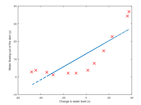
观察图可以拟合的直线为高偏差,因为数据集不是一条直线,而我们现在的数据集X只有一维,不足以拟合成一条曲线。
二:偏差与方差(Bias-variance)
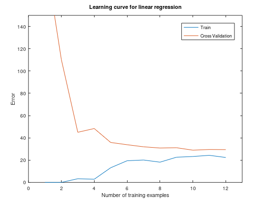
1,学习曲线(Learning curves)
学习曲线将训练和交叉验证误差绘制为训练集大小的函数。
训练集误差(Training error): $J_{train}( heta)=frac{1}{2m}sum_{i=1}^{m}(h_{ heta}(x^{(i)})-y^{(i)})^2$
在计算训练集误差时,在训练子集上进行计算(即$X(1:n,:)$和$y(1:n)$)(而不是整个训练集),
但是,对于交叉验证错误,在整个交叉验证集上对其进行计算。
忽略正则化,我们可视化这个训练集的学习曲线,如下图所示:
function [error_train, error_val] = ...
    learningCurve(X, y, Xval, yval, lambda)
%LEARNINGCURVE Generates the train and cross validation set errors needed
%to plot a learning curve
%   [error_train, error_val] = ...
%       LEARNINGCURVE(X, y, Xval, yval, lambda) returns the train and
%       cross validation set errors for a learning curve. In particular,
%       it returns two vectors of the same length - error_train and
%       error_val. Then, error_train(i) contains the training error for
%       i examples (and similarly for error_val(i)).
%
%   In this function, you will compute the train and test errors for
%   dataset sizes from 1 up to m. In practice, when working with larger
%   datasets, you might want to do this in larger intervals.
%

% Number of training examples
m = size(X, 1);

% You need to return these values correctly
error_train = zeros(m, 1);
error_val   = zeros(m, 1);

% ====================== YOUR CODE HERE ======================
% Instructions: Fill in this function to return training errors in
%               error_train and the cross validation errors in error_val.
%               i.e., error_train(i) and
%               error_val(i) should give you the errors
%               obtained after training on i examples.
%
% Note: You should evaluate the training error on the first i training
%       examples (i.e., X(1:i, :) and y(1:i)).
%
%       For the cross-validation error, you should instead evaluate on
%       the _entire_ cross validation set (Xval and yval).
%
% Note: If you are using your cost function (linearRegCostFunction)
%       to compute the training and cross validation error, you should
%       call the function with the lambda argument set to 0.
%       Do note that you will still need to use lambda when running
%       the training to obtain the theta parameters.
%
% Hint: You can loop over the examples with the following:
%
%       for i = 1:m
%           % Compute train/cross validation errors using training examples
%           % X(1:i, :) and y(1:i), storing the result in
%           % error_train(i) and error_val(i)
%           ....
%
%       end
%

% ---------------------- Sample Solution ----------------------


  for i=1:m

    %给前i个样例拟合参数θ
    theta = trainLinearReg(X(1:i,:), y(1:i,:), lambda);
    %计算前i个样例的训练误差
    [J, grad] = linearRegCostFunction(X(1:i,:), y(1:i,:), theta, 0);
    error_train(i)=J;
    %计算交叉验证集误差
    [J, grad] = linearRegCostFunction(Xval, yval, theta, 0);
    error_val(i)=J;

  end


% -------------------------------------------------------------

% =========================================================================

end
观察此图,可以看到训练集数量增大时,误差还是很大,不会有太大改观,这是属于高偏差/欠拟合(High bias)问题--模型太过于简单,接下来我们将会增加更多的特征去拟合训练集。
2,多项式回归(Polynomial regression)
我们在上一步对于训练集的模型太过于简单,导致出现了欠拟合(高偏差)问题,接下来我们通过原有的特征增加更多新的特征,我们增加p维,每一维为原来特征的i次幂。
回归函数:$h_{ heta}(x)= heta_0+ heta_1(waterLevel)+ heta_2(waterLevel)^{2}+...++ heta_p(waterLevel)^{p}$
$=h_{ heta}(x)= heta_0+ heta_1(x_1)+ heta_2(x_2)^{2}+...++ heta_p(x_p)^{p}$
function [X_poly] = polyFeatures(X, p)
%POLYFEATURES Maps X (1D vector) into the p-th power
%   [X_poly] = POLYFEATURES(X, p) takes a data matrix X (size m x 1) and
%   maps each example into its polynomial features where
%   X_poly(i, :) = [X(i) X(i).^2 X(i).^3 ...  X(i).^p];
%


% You need to return the following variables correctly.
X_poly = zeros(numel(X), p);

% ====================== YOUR CODE HERE ======================
% Instructions: Given a vector X, return a matrix X_poly where the p-th
%               column of X contains the values of X to the p-th power.
%
%

##  for i=1:p
##    X_poly(:,i)=X .^ i;
##  end

for i=1:p
    X_poly(:,i)=X .^ i;
end


% =========================================================================

end
我们增加了新特征之后,要先进行特征缩放。然后我们使用新的训练集去拟合参数$ heta$(忽略正则化)。
此训练集模型的曲线:

将训练集和交叉验证集的代价函数误差与样本数绘制在同一张图表
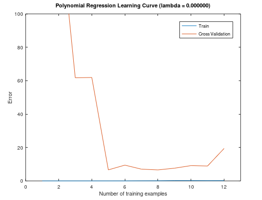
通过以上两图,我们可以看到,该模型完全适合于训练集,但对于交叉验证集,就不能很好的泛化了,此时出现了高方差/过拟合问题。那么接下来我们使用正则化来解决过拟合问题。
3,选择一个合适的正则化参数$lambda$
我们尝试不同的$lambda$值来去选择一个较优的值,例如[0.001,0.003,0.01,0.03,0.1,0.3,1,3,10]
function [lambda_vec, error_train, error_val] = ...
    validationCurve(X, y, Xval, yval)
%VALIDATIONCURVE Generate the train and validation errors needed to
%plot a validation curve that we can use to select lambda
%   [lambda_vec, error_train, error_val] = ...
%       VALIDATIONCURVE(X, y, Xval, yval) returns the train
%       and validation errors (in error_train, error_val)
%       for different values of lambda. You are given the training set (X,
%       y) and validation set (Xval, yval).
%

% Selected values of lambda (you should not change this)
lambda_vec = [0 0.001 0.003 0.01 0.03 0.1 0.3 1 3 10]';

% You need to return these variables correctly.
error_train = zeros(length(lambda_vec), 1);
error_val = zeros(length(lambda_vec), 1);

% ====================== YOUR CODE HERE ======================
% Instructions: Fill in this function to return training errors in
%               error_train and the validation errors in error_val. The
%               vector lambda_vec contains the different lambda parameters
%               to use for each calculation of the errors, i.e,
%               error_train(i), and error_val(i) should give
%               you the errors obtained after training with
%               lambda = lambda_vec(i)
%
% Note: You can loop over lambda_vec with the following:
%
%       for i = 1:length(lambda_vec)
%           lambda = lambda_vec(i);
%           % Compute train / val errors when training linear
%           % regression with regularization parameter lambda
%           % You should store the result in error_train(i)
%           % and error_val(i)
%           ....
%
%       end
%
%

  for i=1:length(lambda_vec)
      lambda=lambda_vec(i);
      [theta] = trainLinearReg(X, y, lambda)
      error_train(i)=linearRegCostFunction(X, y, theta, 0); %计算训练集的误差,忽略正则化的影响
      error_val(i)=linearRegCostFunction(Xval, yval, theta, 0);

  end


% =========================================================================

end
可视化图如下所示:
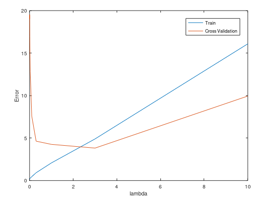
观察图,我们可以选择$lambda=3$。
总结:
1,获得更多的训练实例: 解决高偏差
2,尝试减少特征的数量:解决高方差
3,尝试获得更多的特征: 解决高偏差
4,尝试增加多项式的特征:解决高偏差
5,尝试减少正则化的程度$lambda$:解决高偏差
6,尝试增加正则化的程度$lambda$:解决高方差