构建多层卷积神经网络时需要多组W和偏移项b,我们封装2个方法来产生W和b
初级MNIST中用0初始化W和b,这里用噪声初始化进行对称打破,防止产生梯度0,同时用一个小的正值来初始化b避免dead neurons。
def weight_variable(shape):
    initial = tf.truncated_normal(shape, stddev=0.1)
    return tf.Variable(initial)


def bias_variable(shape):
    initial = tf.constant(0.1, shape=shape)
    return tf.Variable(initial)
tf.truncated_normal()返回truncated normal distribution产生的随机值
def truncated_normal(shape,
                     mean=0.0,
                     stddev=1.0,
                     dtype=dtypes.float32,
                     seed=None,
                     name=None):
stddev:为标准差
mean:为均值
Convolution and Pooling(卷积和池化)
TensorFlow使得convolution和pooling operations具有更多的灵活性,我们怎么处理boundaries,stride size是多少,
这里stride用1,并用0填充使得输入和输出的大小相同。
def conv2d(x, W):
    return tf.nn.conv2d(x, W, strides=[1, 1, 1, 1], padding='SAME')


def max_pool_2x2(x):
    return tf.nn.max_pool(x, ksize=[1, 2, 2, 1], strides=[1, 2, 2, 1], padding='SAME')
卷积函数:
def conv2d(input, filter, strides, padding, use_cudnn_on_gpu=True, data_format="NHWC", name=None):
data_format:string变量,值有 "NHWC", "NCHW"。
    默认为 "NHWC"表示 [batch, height, width, channels]
input:要求为一个4-D Tensor,维度顺序与data_format一样,
    shape为[batch, in_height, in_width, in_channels]
       类型为float32或half
filter:要求为一个4-D Tensor,维度顺序与data_format一样,
shape为[filter_height, filter_width, in_channels, out_channels]
类型与input一样 【 相当于卷积核 】
strides: A list of `ints`或1-D tensor of length 4。对应于input中每一维的滑动窗口
padding:string类型,变量值可取"SAME", "VALID",表示不同的卷积方式
SAME:采用填充的方式
VALID:采用丢弃的方式

具体含义请参考tensorflow conv2d的padding解释以及参数解释
【TensorFlow】tf.nn.conv2d是怎样实现卷积的?
此函数做了哪些事?
1 将filter reshape成2维 [filter_height * filter_weight * in_channels, output_channels]
2 从input中提取image patches,形成虚拟 tensor [batch, out_height, out_width, filter_height * filter_width * in_channels]
3 对于每个batch,右乘 filter matrix和image patch vector
示例:

output[b, i, j, k] =
    sum_{di, dj, q} input[b, strides[1] * i + di, strides[2] * j + dj, q] *
                    filter[di, dj, q, k]

Must have `strides[0] = strides[3] = 1`.  For the most common case of the same
horizontal and vertices strides, `strides = [1, stride, stride, 1]`.
用一个例子来说明:
input的维度为[2, 5, 5, 4]表示batch_size为2, 图片是5 * 5, 输入通道数为 4,
filter的维度为[3, 3, 4, 2]表示卷积核大小为3 * 3,输入通道数为4, 输出通道数为 2
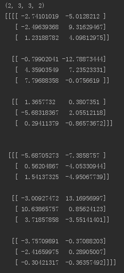
步长为1,padding方式选用VALID
import tensorflow as tf

input = tf.Variable(tf.random_normal([2, 5, 5, 4]))
filter = tf.Variable(tf.random_normal([3, 3, 4, 2]))
op = tf.nn.conv2d(input, filter, strides=[1, 1, 1, 1], padding='VALID')
sess = tf.InteractiveSession()
initializer = tf.global_variables_initializer()
sess.run(initializer)
print(op.shape)
print(sess.run(op))
输出:[batch_size, out_height, out_width, out_channels]
将VALID改为SAME,输出如下:

池化:
pooling通常在convolution 后面,降低卷积层输出的特征向量。
包括max_pool和mean_pool,先介绍max_pool
def max_pool(value, ksize, strides, padding, data_format="NHWC", name=None):
参数介绍:
value:输入通常是feature map(卷积层的输出),依然是一个4-D tensor [batch_size, height, width, channels]
ksize:池化窗口大小,对应value的每一维。一般不在batch_size和channels上池化,所以这2个维度上一般设为1
strides:和卷积类似,窗口在每一个维度上的滑动的步长
padding:和卷积类似,可以取 VALID、SAME
例子说明:
import tensorflow as tf
input = tf.Variable(tf.random_normal([3, 7, 7, 2]))
op = tf.nn.max_pool(input, ksize=[1, 2, 2, 1], strides=[1, 1, 1, 1], padding='VALID')
with tf.Session()as sess:
    sess.run(tf.global_variables_initializer())
    re = sess.run(op)
    print(op.shape)
    print(re)
输出:

以上分别是卷积和池化的介绍,下面开始卷积神经网络的构建。
mnist = input_data.read_data_sets('MNIST_data', one_hot=True)
x = tf.placeholder(tf.float32, shape=(None, 784))
y_ = tf.placeholder(tf.float32, shape=(None, 10))
分别是数据集的下载,以及x,y_的占位
第一层卷积:
卷积会为每5 * 5 patch计算32维的feature
W_conv1 = weight_variable([5, 5, 1, 32])
b_conv1 = bias_variable([32])
x_image = tf.reshape(x, [-1, 28, 28, 1])
h_conv1 = tf.nn.relu(conv2d(x_image, W_conv1) + b_conv1)
h_pool1 = max_pool_2x2(h_conv1)
x_image将x reshape为4-D tensor
max_pool操作将图片size缩为14 * 14
第二层卷积:
为构建深层网络,我们要堆叠多个这种类型的层。第二层每个5 * 5patch有64个feature。
W_conv2 = weight_variable([5, 5, 32, 64])
b_conv2 = bias_variable([64])
h_conv2 = tf.nn.relu(conv2d(h_pool1, W_conv2) + b_conv2)
h_pool2 = max_pool_2x2(h_conv2)
现在图片size为7 * 7
密集连接层
# 密集连接层
W_fcl = weight_variable([7*7*64, 1024])
b_fcl = bias_variable([1024])
h_pool2_flat = tf.reshape(h_pool2, [-1, 7*7*64])
h_fcl = tf.nn.relu(tf.matmul(h_pool2_flat, W_fcl) + b_fcl)
全连接层有1024个神经元,用于处理整个图片
Dropout
请参考理解dropout
为减少过拟合,我们在输出之前应用Dropout,创建一个占位符表示Dropout期间神经元的输出被保留的概率。一般我们可以在training期间打开Dropout,test期间关闭Dropout。
TensorFlow的tf.nn.dropout可以自动缩放神经元的输出并屛蔽它们。
#Dropout层
keep_prob = tf.placeholder(tf.float32)
h_fcl_drop = tf.nn.dropout(h_fcl, keep_prob)
输出层
#输出层
W_fc2 = weight_variable([1024, 10])
b_fc2 = bias_variable([10])
y_conv = tf.matmul(h_fcl_drop, W_fc2) + b_fc2
Train and Evaluate the Model
本节的模型与初级里面的一层softmax网络模型相比有以下不同:
1:用sophisticated ADAM optimizer代替梯度下降法进行优化
2:feed_dict中包含keep_prob来控制丢弃的概率
3:training过程中,每100次迭代输出一次日志
运行:
#loss
cross_entropy = tf.reduce_mean(tf.nn.softmax_cross_entropy_with_logits(logits=y_conv, labels=y_))
train_step = tf.train.AdamOptimizer(1e-4).minimize(cross_entropy)

#eval
correct_prediction = tf.equal(tf.argmax(y_conv, 1), tf.argmax(y_, 1))
accuracy = tf.reduce_mean(tf.cast(correct_prediction, tf.float32))

#run
with tf.Session()as sess:
    sess.run(tf.global_variables_initializer())
    for i in range(20000):
        batch = mnist.train.next_batch(50)
        #train accuracy
        if i % 100 == 0:
            train_accuracy = sess.run(accuracy, feed_dict={x: batch[0], y_: batch[1], keep_prob: 1.0})
            print('step %d,training accuracy %g' % (i, train_accuracy))
        sess.run(train_step, feed_dict={x: batch[0], y_: batch[1], keep_prob: 0.5})
    #test accuracy
    print('test accuracy %g' % sess.run(accuracy, feed_dict={x: mnist.test.images, y_:  mnist.test.labels, keep_prob: 1.0}))
最终test set上的准确率为0.992
完整代码:


from tensorflow.examples.tutorials.mnist import input_data
import tensorflow as tf

mnist = input_data.read_data_sets('MNIST_data', one_hot=True)
x = tf.placeholder(tf.float32, shape=(None, 784))
y_ = tf.placeholder(tf.float32, shape=(None, 10))


def weight_variable(shape):
    initial = tf.truncated_normal(shape, stddev=0.1)
    return tf.Variable(initial)


def bias_variable(shape):
    initial = tf.constant(0.1, shape=shape)
    return tf.Variable(initial)


def conv2d(x, W):
    return tf.nn.conv2d(x, W, strides=[1, 1, 1, 1], padding='SAME')


def max_pool_2x2(x):
    return tf.nn.max_pool(x, ksize=[1, 2, 2, 1], strides=[1, 2, 2, 1], padding='SAME')


# 第一层卷积
W_conv1 = weight_variable([5, 5, 1, 32])
b_conv1 = bias_variable([32])
x_image = tf.reshape(x, [-1, 28, 28, 1])
h_conv1 = tf.nn.relu(conv2d(x_image, W_conv1) + b_conv1)
h_pool1 = max_pool_2x2(h_conv1)

# 第二层卷积
W_conv2 = weight_variable([5, 5, 32, 64])
b_conv2 = bias_variable([64])
h_conv2 = tf.nn.relu(conv2d(h_pool1, W_conv2) + b_conv2)
h_pool2 = max_pool_2x2(h_conv2)

# 密集连接层
W_fcl = weight_variable([7*7*64, 1024])
b_fcl = bias_variable([1024])
h_pool2_flat = tf.reshape(h_pool2, [-1, 7*7*64])
h_fcl = tf.nn.relu(tf.matmul(h_pool2_flat, W_fcl) + b_fcl)

# Dropout层
keep_prob = tf.placeholder(tf.float32)
h_fcl_drop = tf.nn.dropout(h_fcl, keep_prob)

# 输出层
W_fc2 = weight_variable([1024, 10])
b_fc2 = bias_variable([10])
y_conv = tf.matmul(h_fcl_drop, W_fc2) + b_fc2

# loss
cross_entropy = tf.reduce_mean(tf.nn.softmax_cross_entropy_with_logits(logits=y_conv, labels=y_))
train_step = tf.train.AdamOptimizer(1e-4).minimize(cross_entropy)

# eval
correct_prediction = tf.equal(tf.argmax(y_conv, 1), tf.argmax(y_, 1))
accuracy = tf.reduce_mean(tf.cast(correct_prediction, tf.float32))

# run
with tf.Session()as sess:
    sess.run(tf.global_variables_initializer())
    for i in range(20000):
        batch = mnist.train.next_batch(50)
        # train accuracy
        if i % 100 == 0:
            train_accuracy = sess.run(accuracy, feed_dict={x: batch[0], y_: batch[1], keep_prob: 1.0})
            print('step %d,training accuracy %g' % (i, train_accuracy))
        sess.run(train_step, feed_dict={x: batch[0], y_: batch[1], keep_prob: 0.5})
    # test accuracy
    print('test accuracy %g' % sess.run(accuracy, feed_dict={x: mnist.test.images, y_:  mnist.test.labels, keep_prob: 1.0}))
运行结果: