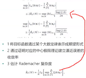
源地址(相关案例在视频下方): http://cookdata.cn/auditorium/course_room/10019/
《机器学习十讲》——第八讲(维度灾难)
维度灾难:随着维度(如特征或自由度)的增多,问题的复杂性(或计算算代价)呈指数级增长的现象。
高维空间的反直觉示例:单位球体积:

一维,二维,三维的 长度/面积/体积 都有公式计算,而高维的计算公式是这样的:
d维空间半径为r的球体体积公式: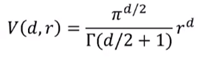
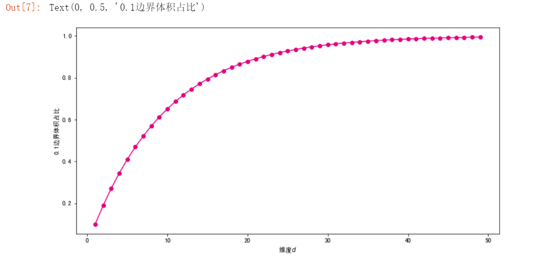
单位球体积与维度之间的关系图示:

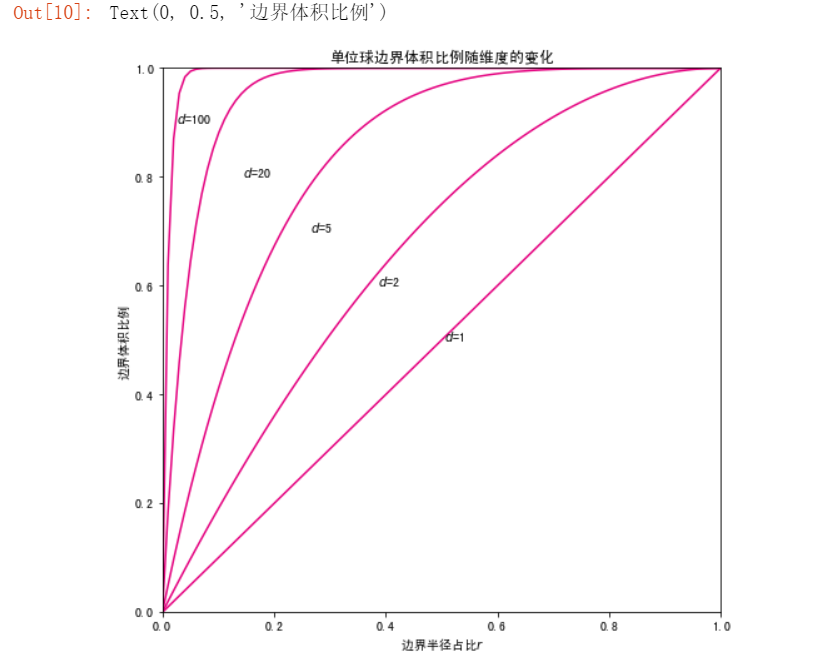
在高维空间中,球体内部的体积与表面积处的体积相比可以忽略不计,大部分体积都是分布在边界的:

高维空间中的欧式距离:d维空间样本x1和x2的欧式距离为: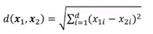
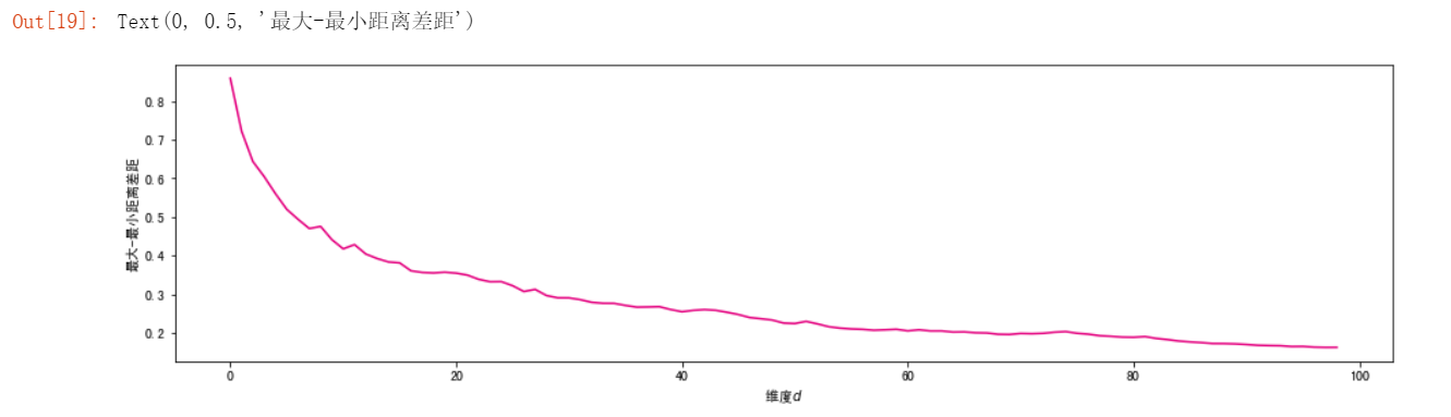
随着维数增加,单个维度对距离的影响越来越小,任意样本间的距离趋于相同:

由于距离在高维空间中不再有效,因此一些基于距离的机器学习模型就会收到影响。
基于距离的机器学习模型:K近邻(样本间距离),支持向量机(样本到决策面距离),K-Means(样本到聚类中心距离),层次聚类(不同簇之间的距离),推荐系统(商品或用户相似度),信息检索(查询和文档之前的相似度)。
稀疏性与过度拟合:
过度拟合:模型对已知数据拟合较好,新的数据拟合较差。极端例子:训练集准确率越来越高,而使用测试集测试模型准确率依然维持在0.5左右。
稀疏性:高维空间中样本变得极度稀疏,容易会造成过度拟合问题。
Hughes现象:随着维度增大,分类器性能不断提升直到达到最佳维度,继续增加维度分类器性能会下降。
高维空间计算复杂度指数增长,因此只能近似求解,得到局部最优解而非全局最优解。
举例——决策树:选择切分点对空间进行划分。每个特征m个取值,候选划分数量m^d(维度灾难)
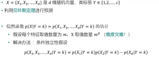
举例——朴素贝叶斯:
应对维度灾难:特征选择和降维
特征选择:选取特征子集。
降维:使用一定变换,将高维数据转换为低维数据,PCA,流形学习,t-SNE等。
正则化:减少泛化误差而不是训练误差

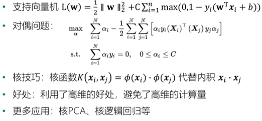
核技巧:
判断机器学习模型是否存在维度灾难问题:
不存在维度灾难问题的模型:随机特征模型,两层神经网络,残差神经网络等
案例——使用Python认识维度问题。
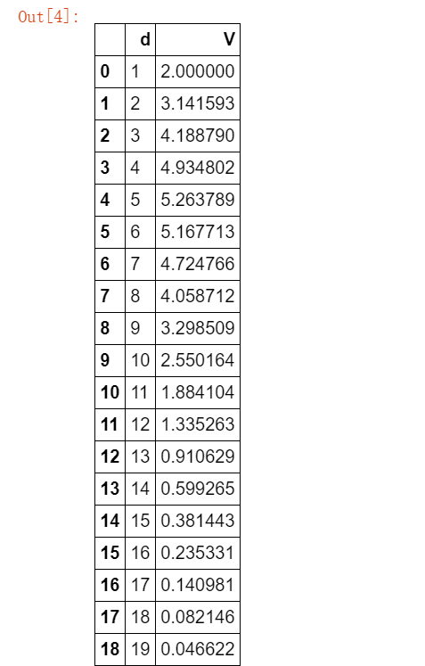
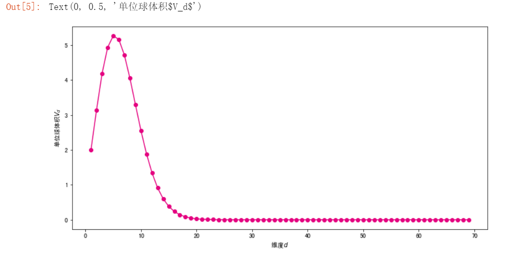
单位球体积随着维度的变化

#公式实现
import numpy as np
import math
#引用伽马函数
from scipy.special import gamma
def V(d,r):
    return math.pi**(d/2)*(r**d)/gamma(d/2 + 1)
#测试一下
print(V(1,1))
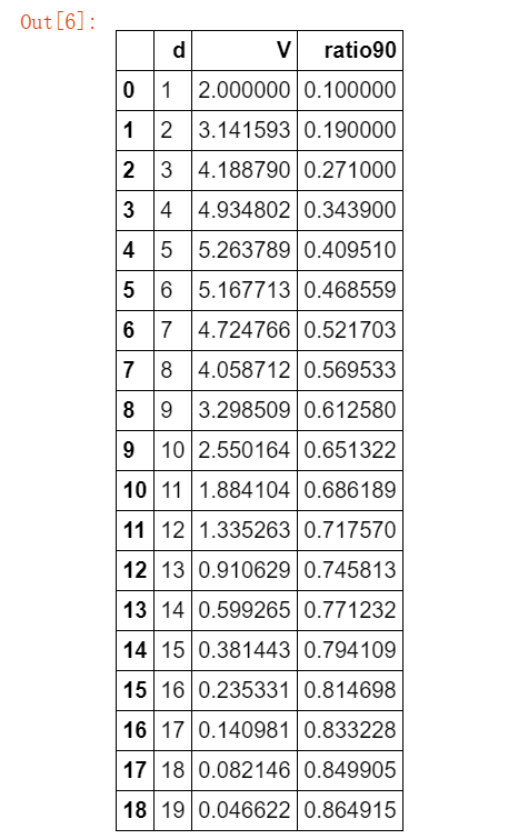
#使用公式计算1-20维单位球的体积
import pandas as pd
df = pd.DataFrame()
df["d"] = np.arange(1,20)
#半径为1
df["V"] = V(df["d"],1)
df.round(9)
#将单位球体积随着维度的变化进行可视化
##为了方便观察,设置维度为1-70
import matplotlib.pyplot as plt
%matplotlib inline
fig, ax = plt.subplots(figsize=(12, 6)) #设置图片大小
ds = np.arange(1,70)
plt.plot(ds,V(ds,1),color="#E4007F",marker="o")
plt.xlabel("维度$d$")
plt.ylabel("单位球体积$V_d$")
#看一下0.1半径体积的比例是多少
##假设边界为0.1
def ratio(d):
    return (V(d,1) - V(d,0.9))/ V(d,1)
df["ratio90"] =  1 - 0.9**(df.d)
df.round(6).head(20)
#将0.1边界体积比例可视化
import matplotlib.pyplot as plt
%matplotlib inline
fig, ax = plt.subplots(figsize=(12, 6)) #设置图片大小
ds = np.arange(1,50)
plt.plot(ds,ratio(ds),color="#E4007F",marker="o")
plt.xlabel("维度$d$")
plt.ylabel("0.1边界体积占比")
#刚才的方法是指定边界为0.1,为了能查看任意边界比例的情况,再写一个方法
def volumn_fraction_in_border(d,r):
    return(V(d,1)-V(d,1-r))/V(d,1)
#可视化
import numpy as np
#设置维度
ds=[1,2,5,20,100]
#设置颜色
colors=["gray","#E4007F","","","",""]
rs=np.linspace(0,1,100)
result=[]
for d in ds:
    vs=[]
    for r in rs:
        vs.append(volumn_fraction_in_border(d,r))
    result.append(vs)
import matplotlib.pyplot as plt
%matplotlib inline
fig, ax = plt.subplots(figsize=(8, 8)) #设置图片大小
plt.title("单位球边界体积比例随维度的变化")
for i in range(len(ds)):
    plt.plot(rs,result[i],color="#E4007F",label="d="+str(ds[i]))
    plt.text(rs[50]-i*0.12,0.5+i*0.1,"$d$="+str(ds[i]))
plt.xlim(0,1)
plt.ylim(0,1)
plt.xlabel("边界半径占比$r$")
plt.ylabel("边界体积比例")
高维空间中的样本距离

#定义方法计算欧式距离
def data_euclidean_dist(x):
    sum_x = np.sum(np.square(x), 1)
    dist = np.add(np.add(-2 * np.dot(x, x.T), sum_x).T, sum_x)
    return dist
#自定义一个矩阵,计算两两之间的欧式距离
x = np.array([[0, 1, 3], [3, 8, 9], [2, 3, 5]])
dist_matrix = data_euclidean_dist(x)
dist_matrix
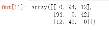
#使用mask去掉对角线(0)
##计算该欧式距离中的最小值
mask = np.ones(dist_matrix.shape, dtype=bool)
np.fill_diagonal(mask, 0)
dist_matrix[mask].min()

#生成一个包含5000个样本5000个维度的数据集。每一个维度都是从[-1,1]之间随机生成。
X = np.random.uniform(-1,1,(5000,5000))
#显示
X
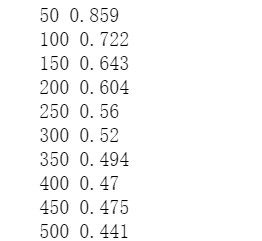
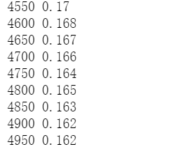
#求随着维度增大,样本间欧式距离最大值与最小值的差值,需要用mask去掉对角0
min_max_list = []
#设置间隔为50
for d in range(50,5000,50):
    dist_matrix = data_euclidean_dist(X[:,:d])
    mask = np.ones(dist_matrix.shape, dtype=bool)
    np.fill_diagonal(mask, 0)
    min_max = (dist_matrix[mask].max() - dist_matrix[mask].min())/dist_matrix[mask].max()
    if d%50 == 0:
        print(d,min_max.round(3))
    min_max_list.append(min_max)
#可视化
import matplotlib.pyplot as plt
%matplotlib inline
fig, ax = plt.subplots(figsize=(16, 4)) #设置图片大小
ds = np.arange(0,len(min_max_list))
plt.plot(ds,min_max_list,color="#E4007F")
plt.xlabel("维度$d$")
plt.ylabel("最大-最小距离差距")
维度对分类性能的影响

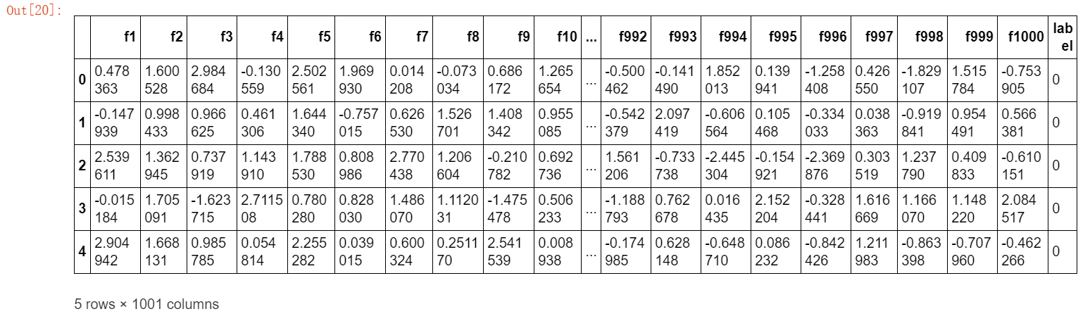
#生成Trunk数据集
import pandas as pd
import numpy as np
max_features,num_samples = 1000,500 #最大特征数量和样本数量
X_pos = pd.DataFrame()
X_neg = pd.DataFrame()

for i in range(max_features):
    X_pos["f"+str(i+1)] = np.random.randn(num_samples)+ np.sqrt(1/(i+1)) #生成当前特征的正类样本
    X_neg["f"+str(i+1)] = np.random.randn(num_samples)- np.sqrt(1/(i+1)) #生成当前特征的负类样本

X_pos["label"],X_neg["label"] = 0,1 #添加标签
trunk_data = pd.concat([X_pos,X_neg],axis=0) #合并正类和负类样本
trunk_data.head()
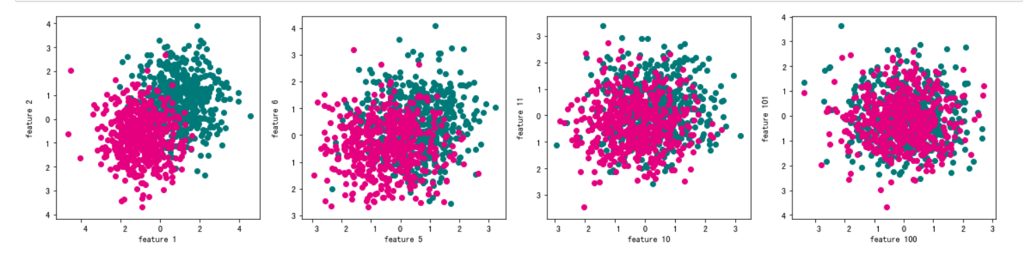
#随机选择几个特征,用散点图可视化正负类样本的分布情况。
import matplotlib.pyplot as plt
%matplotlib inline
features = [1,5,10,100]
fig, ax = plt.subplots(figsize=(16, 4)) #设置图片大小

for i in range(len(features)):
    plt.subplot(1,4,i+1)
    plt.scatter(trunk_data[trunk_data.label == 0]["f" + str(features[i])], trunk_data[trunk_data.label == 0]["f" + str(features[i]+1)], color="#007979")
    plt.scatter(trunk_data[trunk_data.label == 1]["f" + str(features[i])], trunk_data[trunk_data.label == 1]["f" + str(features[i]+1)],color="#E4007F")
    plt.xlabel("feature " + str(features[i]))
    plt.ylabel("feature " + str(features[i]+1))
plt.tight_layout()
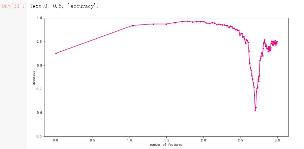
#不断增加特征数量,观察分类性能随着维数的变化。
from sklearn.model_selection import train_test_split
X_train,X_test,y_train,y_test = train_test_split(trunk_data.iloc[:,:-1],trunk_data["label"],test_size=0.5)#训练集和测试集划分
from sklearn.discriminant_analysis import LinearDiscriminantAnalysis
num_features = np.arange(1,max_features,10)
exp_times = 10 #试验次数
test_result = np.zeros(len(num_features))
train_result = np.zeros(len(num_features))
#实验用到不同维度,所以使用两层for循环控制
for t in range(exp_times): #运行多次试验
    scores_train = [] #记录训练集正确率
    scores_test = [] #记录测试集正确率
    for num_feature in num_features:  #使用不同特征数量
        clf = LinearDiscriminantAnalysis()#新建分类模型
        clf.fit(X_train.iloc[:,:num_feature],y_train)#用训练集对应特征数去训练
        score_train = clf.score(X_train.iloc[:,:num_feature],y_train)#记录训练集正确率
        score_test = clf.score(X_test.iloc[:,:num_feature],y_test)#记录测试集正确率
        scores_train.append(score_train)
        scores_test.append(score_test)
    train_result += np.array(scores_train)
    test_result += np.array(scores_test)
    print(t)
#求平均值
test_result /= exp_times
train_result /= exp_times

#训练好后进行可视化
fig, ax = plt.subplots(figsize=(12, 6))
ax.plot(np.log10(num_features),test_result,color="#E4007F",marker=".")
plt.ylim(0.5,1)
plt.xlabel("number of features")
plt.ylabel("accuracy")
使用高维处理非线性问题
维度的好处:
#生成一份月牙形随机线性不可分随机数据集。
import pandas as pd
from sklearn import datasets
sample,target = datasets.make_moons(n_samples=300,shuffle=True,noise=0.1,random_state=0)
data = pd.DataFrame(data=sample,columns=["x1","x2"])
data["label"] = target
#可视化
import matplotlib.pyplot as plt
%matplotlib inline
plt.rcParams['axes.unicode_minus']=False  # 用来正常显示负号
fig, ax = plt.subplots(figsize=(6, 6)) #设置图片大小
ax.scatter(data[data.label==0]["x1"],data[data.label==0]["x2"],color="#007979")
ax.scatter(data[data.label==1]["x1"],data[data.label==1]["x2"],color="#E4007F")
plt.xlabel("$x_1$")
plt.ylabel("$x_2$")

#使用线性支持向量机进行分类。
from sklearn.model_selection import train_test_split
X_train,X_test,y_train,y_test = train_test_split(data[["x1","x2"]],data.label,test_size=0.5)
#获取参数
from sklearn.svm import LinearSVC
svm_linear = LinearSVC()
svm_linear.fit(X_train,y_train)
svm_linear.score(X_test,y_test)
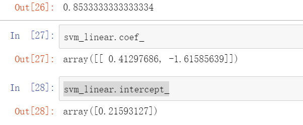
#将决策直线画出来
fig, ax = plt.subplots(figsize=(6, 6)) #设置图片大小
ax.scatter(X_train[y_train==0]["x1"],X_train[y_train==0]["x2"],color="#007979")
ax.scatter(X_train[y_train==1]["x1"],X_train[y_train==1]["x2"],color="#E4007F")
ax.scatter(X_test[y_test==0]["x1"],X_test[y_test==0]["x2"],color="#007979",marker="^",alpha=0.6)
ax.scatter(X_test[y_test==1]["x1"],X_test[y_test==1]["x2"],color="#E4007F",marker="^",alpha=0.6)
x1 = np.linspace(-1.5,2.5,50)
x2 = - x1*svm_linear.coef_[0][0]/svm_linear.coef_[0][1] - svm_linear.intercept_[0]/svm_linear.coef_[0][1]
ax.plot(x1,x2,color="gray")
plt.xlabel("$x_1$")
plt.ylabel("$x_2$")

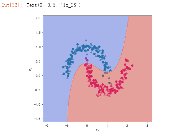
#使用带有核函数的支持向量机模型
from sklearn.svm import SVC
#rbf核函数
svm_rbf = SVC(kernel='rbf')
svm_rbf.fit(X_train,y_train)
svm_rbf.score(X_test,y_test)

#绘制分类决策面的辅助函数,代码来源于Sklearn官网
##网址:https://scikit-learn.org/stable/auto_examples/svm/plot_iris_svc.html
def plot_contours(ax, clf, xx, yy, **params):
    Z = clf.predict(np.c_[xx.ravel(), yy.ravel()])
    Z = Z.reshape(xx.shape)
    out = ax.contourf(xx, yy, Z, **params)
    return out
def make_meshgrid(x, y, h=.02):
    x_min, x_max = x.min() - 1, x.max() + 1
    y_min, y_max = y.min() - 1, y.max() + 1
    xx, yy = np.meshgrid(np.arange(x_min, x_max, h),np.arange(y_min, y_max, h))
    return xx, yy
#绘制决策平面
xx, yy = make_meshgrid(X_train["x1"], X_train["x2"])

fig, ax = plt.subplots(figsize=(6, 6)) #设置图片大小
ax.scatter(X_train[y_train==0]["x1"],X_train[y_train==0]["x2"],color="#007979")
ax.scatter(X_train[y_train==1]["x1"],X_train[y_train==1]["x2"],color="#E4007F")
ax.scatter(X_test[y_test==0]["x1"],X_test[y_test==0]["x2"],color="#007979",marker="^",alpha=0.6)
ax.scatter(X_test[y_test==1]["x1"],X_test[y_test==1]["x2"],color="#E4007F",marker="^",alpha=0.6)

plot_contours(ax, svm_rbf, xx, yy, cmap=plt.cm.coolwarm, alpha=0.5)

plt.xlabel("$x_1$")
plt.ylabel("$x_2$")
维度的弊端,这里展示的是过度拟合:
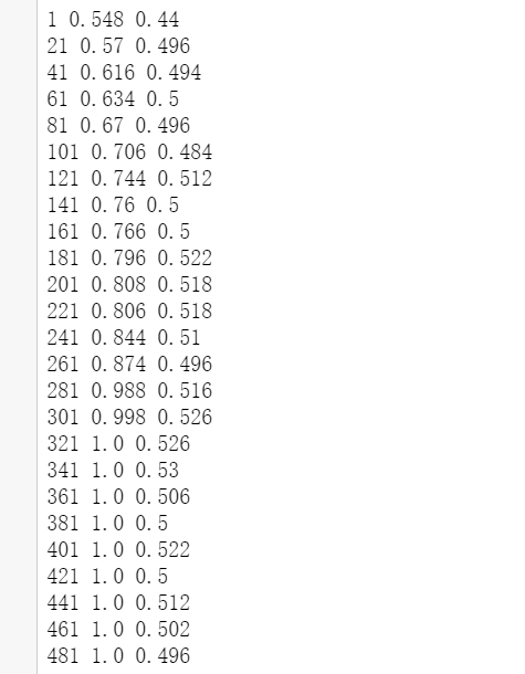
#随机生成一份满足标准正态分布的数据集,包含1000个样本,500个特征。类别标签是从0和1中随机生成的
#等分成训练集和测试集(1:1)
X = np.random.randn(1000,500) #生成满足标准正太分布的特征
y = np.random.randint(0,2,1000) #生成标签
X_train,X_test,y_train,y_test = train_test_split(X,y,test_size=0.5)#训练集和测试集划分
#借助线性支持向量机模型,断增大使用的特征数量,观察模型在训练集和测试集上的正确率变化情况。
from sklearn.svm import LinearSVC
num_features = np.arange(1,X.shape[1],20)
scores_train = [] #记录训练集正确率
scores_test = [] #记录测试集正确率
for num_feature in num_features:
    linear_svm = LinearSVC() #新建线性支持向量机
    linear_svm.fit(X_train[:,:num_feature],y_train)
    score_train = linear_svm.score(X_train[:,:num_feature],y_train)
    score_test = linear_svm.score(X_test[:,:num_feature],y_test)
    scores_train.append(score_train)
    scores_test.append(score_test)
    print(num_feature,score_train,score_test)
#可视化
fig, ax = plt.subplots(figsize=(8, 6)) #设置图片大小
ax.plot(num_features,scores_train,color="#007979",marker="o")
ax.plot(num_features,scores_test,color="#E4007F",marker="^")
ax.hlines(0.5,0,500,color="gray",linestyles="--")
plt.ylim(0,1.2)
plt.xlabel("number of features")
plt.ylabel("accuracy")
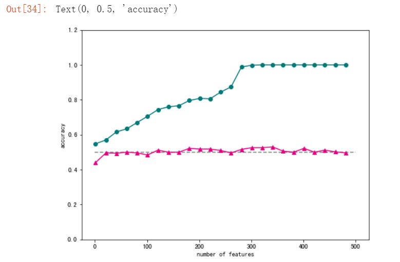
可见测试集中正确率依然维持在0.5左右。发生了过度拟合。