机器人定位问题
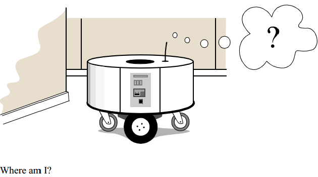
General schematic for mobile robot localization

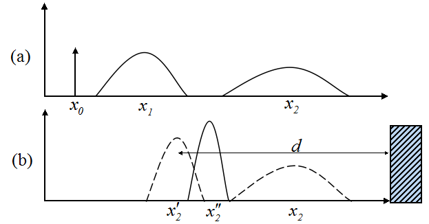
以下面的两幅图a、b为例,对移动机器人定位问题进行说明。假如机器人从一个已知的位置开始运动,利用里程计(编码器)可以对其运动进行跟踪,由于里程计的误差,运动一段时间后,机器人对其位置的不确定度将变得很大。为了使位置的不确定性不至于无限增大,机器人必须参考其外部环境对自己进行定位。为了进行定位,机器人会使用外部传感器(例如,超声、激光、视觉传感器等)对环境进行测量。如下图a所示的预测阶段:起始位置x0已知,所以该位置上概率密度函数是δ函数(狄拉克函数)。当机器人开始移动,由于里程计的误差,它的不确定性增加,并随时间积累(In short, mobile robot effectors introduce uncertainty about future state. Therefore the simple act of moving tends to increase the uncertainty of a mobile robot)。下图b所示为感知阶段:机器人利用外部传感器测量到右墙的距离为d,计算出当前位置为x'2,这与预测的位置x2有冲突。融合两个估计的概率密度,将位置校正,其不确定性得到减小(图b中的实线)。
The MCL Algorithm
1. Randomly generate a bunch of particles
Particles can have position, heading, and/or whatever other state variable you need to estimate. Each has a weight (probability) indicating how likely it matches the actual state of the system. Initialize each with the same weight.
2. Predict next state of the particles
Move the particles based on how you predict the real system is behaving.
3. Update
Update the weighting of the particles based on the measurement. Particles that closely match the measurements are weighted higher than particles which don't match the measurements very well.
4. Resample
Discard highly improbable particle and replace them with copies of the more probable particles.
5. Compute Estimate
Optionally, compute weighted mean and covariance of the set of particles to get a state estimate.
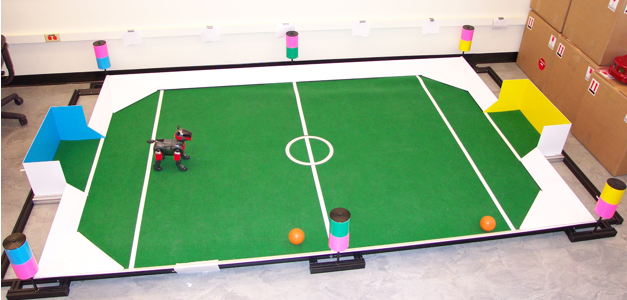
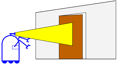
粒子滤波定位又称为蒙特卡罗定位(MCL, or Monte Carlo Localization, a localization algorithm based on particle filters)。粒子滤波的基本步骤为上面所述的5步,其本质是使用一组有限的加权随机样本(粒子)来近似表征任意状态的后验概率密度。粒子滤波的优势在于对复杂问题的求解上,比如高度的非线性、非高斯动态系统的状态递推估计或概率推理问题。下面考虑一个2维平面内机器人定位的问题。机器人定位技术可分为相对定位和绝对定位两类。相对定位是通过测量机器人相对于初始位置的距离和方向来确定机器人的当前位置,通常称为航迹推算法,常用的传感器包括里程计及惯性导航系统(陀螺仪、加速度计等);绝对定位主要采用导航信标、主动或被动标识、地图匹配或卫星导航技术进行定位。下图中的机器人采用路标定位,路标一般定义为环境中被动的物体,当它们处在机器人传感器测量范围内时,提供了高的定位准确度。基于路标的导航中,一般路标都有固定的已知位置,机器人自身传感器能对路标进行识别,通过与路标间的相对定位实现机器人在地图中的绝对定位。如下图所示,机器人通过视觉传感器识别球场边上用特定颜色标记的柱子(landmarks)来定位。
基本的MCL算法步骤如下:
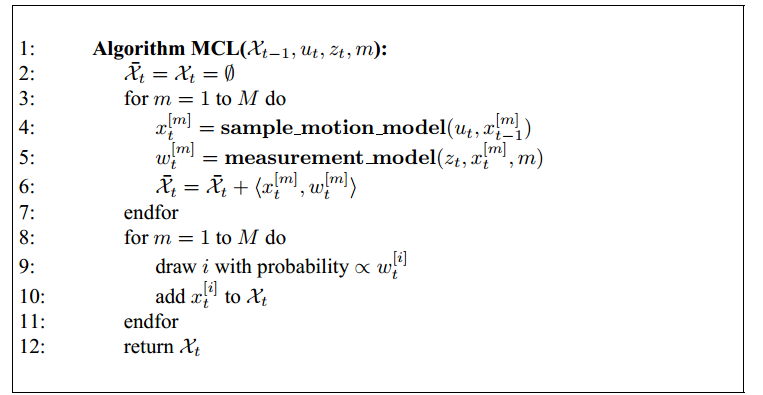
即用M个粒子来描述状态向量的后验概率分布。算法第4行从系统转移模型中取样,将这些取样的粒子作为先验值。第5行使用测量模型修正粒子的权值。下面举一个简单的例子,来理解MCL算法:
如下图(a)所示,机器人在水平方向沿一维直线移动。为了推测自身位置,初始时刻在其运动范围内随机生成均匀分布的粒子。粒子的X轴坐标表示推测的机器人位置,Y坐标表示处于这个位置的概率。机器人通过传感器探测门时,按照算法第5行,MCL将修正每个粒子的权值。结果如图(b)所示,可以看到与测量结果接近的粒子被赋予更大的权值。这里要注意,与图(a)相比粒子的X坐标并未被改变,改变的只是权值。

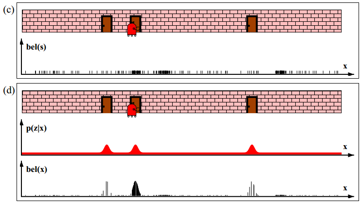
图(c)为重采样后的粒子分布(line 8-11 in the algorithm MCL). This leads to a new particle set with uniform importance weights, but with an increased number of particles near the three likely places. 即重采样后粒子权值归一,但是在机器人可能出现的位置处,粒子数目开始变多。接下来再进行测量校正,如图(d)所示。At this point, most of the cumulative probability mass is centered on the second door, which is also the most likely location.
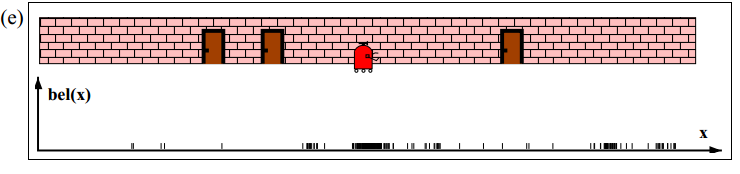
Further motion leads to another resampling step, and a step in which a new particle set is generated according to the motion model (Figure 8.11e). As should be obvious from this example, the particle sets approximate the correct posterior, as would be calculated by an exact Bayes filter.
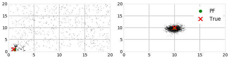
下面我们来看一个2维平面上的例子,机器人在二维平面上移动,其转向和速度作为控制输入信号,机器人自身传感器可以测量其与地图中4个路标之间的距离。下面左图是采用粒子滤波法估计机器人位置的第一次迭代,右图为第10次迭代,图中红色的'X'表示小车真实位置,红色圆圈表示粒子滤波计算出的位置。
下面的动态图显示了粒子滤波的整个过程:

从图中可以看出第一次迭代后粒子仍然大量随机的分散在地图中,但是有一部分粒子已经开始聚集在小车的位置处。粒子滤波算出的结果与小车位置接近,这是因为离测量结果越接近的粒子赋予的权重越大,比如当小车运动到坐标(1,1)时,离(1,1)越近的点权值越大。小车位置的估计值通过粒子的加权平均计算出来,离小车真实值越近的粒子在估计中所占的比重越大。
步骤1:生成粒子
为了估计机器人真实位置,我们选取机器人位置x,y和其朝向θ作为状态变量,因此每个粒子需要有三个特征。用矩阵particles存储N个粒子信息,其为N行3列的矩阵。下面的代码可以在一个区域上生成服从均匀分布的粒子或服从高斯分布的粒子:
 1 from numpy.random import uniform,randn
 2
 3 def create_uniform_particles(x_range, y_range, hdg_range, N):
 4     particles = np.empty((N, 3))
 5     particles[:, 0] = uniform(x_range[0], x_range[1], size=N)
 6     particles[:, 1] = uniform(y_range[0], y_range[1], size=N)
 7     particles[:, 2] = uniform(hdg_range[0], hdg_range[1], size=N)
 8     particles[:, 2] %= 2 * np.pi
 9     return particles
10
11 def create_gaussian_particles(mean, std, N):
12     particles = np.empty((N, 3))
13     particles[:, 0] = mean[0] + (randn(N) * std[0])
14     particles[:, 1] = mean[1] + (randn(N) * std[1])
15     particles[:, 2] = mean[2] + (randn(N) * std[2])
16     particles[:, 2] %= 2 * np.pi
17     return particles
步骤2:利用系统模型预测状态
每一个粒子都代表了一个机器人的可能位置,假设我们发送控制指令让机器人移动0.1米,转动0.7弧度,我么可以让每个粒子移动相同的量。由于控制系统存在噪声,因此需要添加合理的噪声。
 1 def predict(particles, u, std, dt=1.):
 2     """ move according to control input u (heading change, velocity)
 3     with noise Q (std heading change, std velocity)`"""
 4
 5     N = len(particles)
 6     # update heading
 7     particles[:, 2] += u[0] + (randn(N) * std[0])
 8     particles[:, 2] %= 2 * np.pi
 9
10     # move in the (noisy) commanded direction
11     dist = (u[1] * dt) + (randn(N) * std[1])
12     particles[:, 0] += np.cos(particles[:, 2]) * dist
13     particles[:, 1] += np.sin(particles[:, 2]) * dist
步骤3:更新粒子权值
使用测量数据(机器人距每个路标的距离)来修正每个粒子的权值,保证与真实位置越接近的粒子获得的权值越大。由于机器人真实位置是不可测的,可以看作一个随机变量。根据贝叶斯公式可以称机器人在位置x处的概率P(x)为先验分布密度(prior),或预测值,预测过程是利用系统模型(状态方程)预测状态的先验概率密度,也就是通过已有的先验知识对未来的状态进行猜测。在位置x处获得观测量z的概率P(z|x)为似然函数(likelihood)。后验概率为P(x|z), 即根据观测值z来推断机器人的状态x。更新过程利用最新的测量值对先验概率密度进行修正,得到后验概率密度,也就是对之前的猜测进行修正。
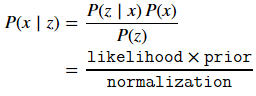
贝叶斯定理中的分母P(z)不依赖于x,因此,在贝叶斯定理中因子P(z)-1常写成归一化因子η。
可以看出,在没有测量数据可利用的情况下,只能根据以前的经验对x做出判断,即只是用先验分布P(x);但如果获得了测量数据,则可以根据贝叶斯定理对P(x)进行修正,即将先验分布与实际测量数据相结合得到后验分布。后验分布是测量到与未知参数有关的实验数据之后所确定的分布,它综合了先验知识和测量到的样本知识。因此基于后验分布对未知参数做出的估计较先验分布而言更有合理性,其估计的误差也较小。这是一个将先验知识与测量数据加以综合的过程,也是贝叶斯理论具有优越性的原因所在。
贝叶斯滤波递推的基本步骤如下:
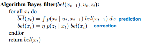
式子中概率p(xt|ut,xt-1)是机器人的状态转移概率,它描述了机器人在控制量ut的作用下从前一个状态xt-1转移到下一状态xt的概率( It describes how much the x changes over one time step)。 由于真实环境的复杂性(比如控制存在误差、噪声或模型不够准确),机器人根据理论模型推导下一时刻的状态时,只能由概率分布p(xt|ut,xt-1)来描述,而非准确无误的量。参考Probabilistic Robotics中的一个例子:t-1时刻门处于关闭状态,然后在控制量Ut的作用下机器人去推门,则t时刻门被推开的概率为0.8,没有被推开的概率为0.2
p(Xt = open | Ut = push, Xt-1 = closed) = 0.8
p(Xt = closed | Ut = push, Xt-1 = closed) = 0.2
然而一般情况下,概率p(xt|ut,xt-1)及p(zt|xt)的分布是未知的,仅对某些特定的动态系统可求得后验概率密度的解析解。比如当p(x0),p(xt|ut,xt-1)及p(zt|xt)都为高斯分布时,后验概率密度仍为高斯分布,并可由此推导出标准卡尔曼滤波。
这一步是非常关键的一步,即如何根据预测值和测量值修正粒子的权值。函数update的参数particles可以看做先验概率分布p(xt|ut,xt-1)的取样值。假设传感器噪声符合高斯分布,那么在位置xt处获得观测量zt的概率p(zt|xt)可以由scipy.stats.norm(dist, R).pdf(z[i])来描述。由于多个路标特征之间的观测相互独立,因此符合概率乘法公式的条件,即下面代码第5行中的累乘。
1 def update(particles, weights, z, R, landmarks):
2     weights.fill(1.)
3     for i, landmark in enumerate(landmarks):
4         dist = np.linalg.norm(particles[:, 0:2] - landmark, axis=1)
5         weights *= scipy.stats.norm(dist, R).pdf(z[i])
6
7     weights += 1.e-300      # avoid round-off to zero
8     weights /= sum(weights) # normalize
步骤4:重采样
在计算过程中,经过数次迭代,只有少数粒子的权值较大,其余粒子的权值可以忽略不计,粒子权值的方差随着时间增大,状态空间中的有效粒子数目减少,这一问题称为权值退化问题。随着无效粒子数目的增加,大量计算浪费在几乎不起作用的粒子上,使得估计性能下降。通常采用有效粒子数Neff衡量粒子权值的退化程度。Neff的近似计算公式为:
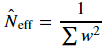
有效粒子数越小,表明权值退化越严重。当Neff的值小于某一阈值时,应当采取重采样措施,根据粒子权值对离散粒子进行重采样。重采样方法舍弃权值较小的粒子,代之以权值较大的粒子,有点类似于遗传算法中的“适者生存”原理。重采样的方法包括多项式重采样(Multinomial resampling)、残差重采样(Residual resampling)、分层重采样(Stratified resampling)和系统重采样(Systematic resampling)等。重采样带来的新问题是,权值越大的粒子子代越多,相反则子代越少甚至无子代。这样重采样后的粒子群多样性减弱,从而不足以用来近似表征后验密度。克服这一问题的方法有多种,最简单的就是直接增加足够多的粒子,但这常会导致运算量的急剧膨胀。其它方法可以去查看有关文献,这里暂不做介绍。
重采样的基本步骤如下:
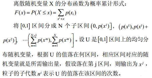

简单的多项式重采样(Multinomial resampling)代码如下:
 1 def simple_resample(particles, weights):
 2     N = len(particles)
 3     cumulative_sum = np.cumsum(weights)
 4     cumulative_sum[-1] = 1. # avoid round-off error
 5     indexes = np.searchsorted(cumulative_sum, random(N))
 6
 7     # resample according to indexes
 8     particles[:] = particles[indexes]
 9     weights[:] = weights[indexes]
10     weights /= np.sum(weights) # normalize
步骤5:计算状态变量估计值
系统状态变量估计值可以通过粒子群的加权平均值计算出来。
1 def estimate(particles, weights):
2     """returns mean and variance of the weighted particles"""
3
4     pos = particles[:, 0:2]
5     mean = np.average(pos, weights=weights, axis=0)
6     var  = np.average((pos - mean)**2, weights=weights, axis=0)
7     return mean, var
下面是完整的程序:


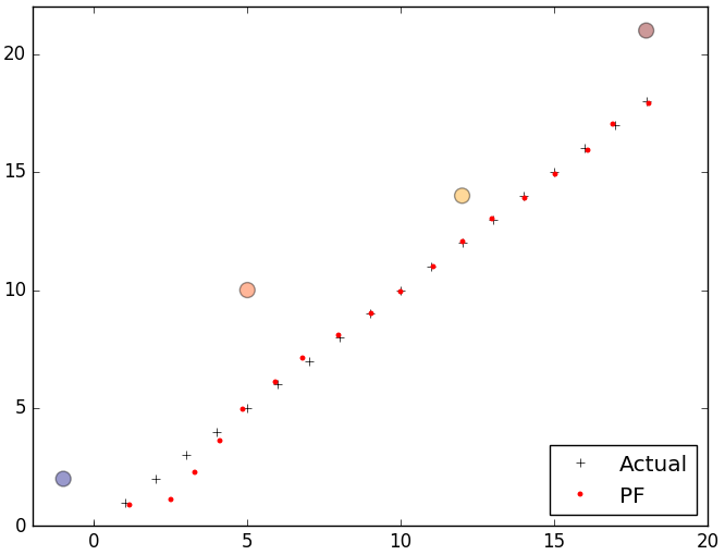
import numpy as np
import scipy.stats
from numpy.random import uniform,randn,random
import matplotlib.pyplot as plt


def create_uniform_particles(x_range, y_range, hdg_range, N):
    particles = np.empty((N, 3))
    particles[:, 0] = uniform(x_range[0], x_range[1], size=N)
    particles[:, 1] = uniform(y_range[0], y_range[1], size=N)
    particles[:, 2] = uniform(hdg_range[0], hdg_range[1], size=N)
    particles[:, 2] %= 2 * np.pi
    return particles


def predict(particles, u, std, dt=1.):
    """ move according to control input u (heading change, velocity)
    with noise Q (std heading change, std velocity)"""

    N = len(particles)
    # update heading
    particles[:, 2] += u[0] + (randn(N) * std[0])
    particles[:, 2] %= 2 * np.pi

    # move in the (noisy) commanded direction
    dist = (u[1] * dt) + (randn(N) * std[1])
    particles[:, 0] += np.cos(particles[:, 2]) * dist
    particles[:, 1] += np.sin(particles[:, 2]) * dist


def update(particles, weights, z, R, landmarks):
    weights.fill(1.)
    for i, landmark in enumerate(landmarks):
        distance = np.linalg.norm(particles[:, 0:2] - landmark, axis=1)
        weights *= scipy.stats.norm(distance, R).pdf(z[i])

    weights += 1.e-300      # avoid round-off to zero
    weights /= sum(weights) # normalize


def estimate(particles, weights):
    """returns mean and variance of the weighted particles"""

    pos = particles[:, 0:2]
    mean = np.average(pos, weights=weights, axis=0)
    var  = np.average((pos - mean)**2, weights=weights, axis=0)
    return mean, var


def neff(weights):
    return 1. / np.sum(np.square(weights))


def simple_resample(particles, weights):
    N = len(particles)
    cumulative_sum = np.cumsum(weights)
    cumulative_sum[-1] = 1. # avoid round-off error
    indexes = np.searchsorted(cumulative_sum, random(N))

    # resample according to indexes
    particles[:] = particles[indexes]
    weights[:] = weights[indexes]
    weights /= np.sum(weights) # normalize


def run_pf(N, iters=18, sensor_std_err=0.1, xlim=(0, 20), ylim=(0, 20)):
    landmarks = np.array([[-1, 2], [5, 10], [12,14], [18,21]])
    NL = len(landmarks)

    # create particles and weights
    particles = create_uniform_particles((0,20), (0,20), (0, 2*np.pi), N)
    weights = np.zeros(N)

    xs = []   # estimated values
    robot_pos = np.array([0., 0.])

    for x in range(iters):
        robot_pos += (1, 1)

        # distance from robot to each landmark
        zs = np.linalg.norm(landmarks - robot_pos, axis=1) + (randn(NL) * sensor_std_err)

        # move particles forward to (x+1, x+1)
        predict(particles, u=(0.00, 1.414), std=(.2, .05))

        # incorporate measurements
        update(particles, weights, z=zs, R=sensor_std_err, landmarks=landmarks)

        # resample if too few effective particles
        if neff(weights) < N/2:
            simple_resample(particles, weights)

        # Computing the State Estimate
        mu, var = estimate(particles, weights)
        xs.append(mu)

    xs = np.array(xs)
    plt.plot(np.arange(iters+1),'k+')
    plt.plot(xs[:, 0], xs[:, 1],'r.')
    plt.scatter(landmarks[:,0],landmarks[:,1],alpha=0.4,marker='o',c=randn(4),s=100) # plot landmarks
    plt.legend( ['Actual','PF'], loc=4, numpoints=1)
    plt.xlim([-2,20])
    plt.ylim([0,22])
    print 'estimated position and variance:
	', mu, var
    plt.show()


if __name__ == '__main__':
    run_pf(N=5000)
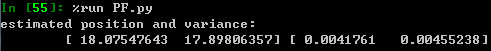
图中4个颜色各异的大圆点是路标,红色小圆点是粒子滤波估计出的机器人位置:
参考:
Probabilistic Robotics chapter 8 p200
https://github.com/rlabbe/Kalman-and-Bayesian-Filters-in-Python
http://www.cs.utexas.edu/~teammco/misc/particle_filter/
Particle Filter Tutorial 粒子滤波:从推导到应用(一)