基于自动编码机(autoencoder),这里网络的层次结构为一个输入层,两个隐层,后面再跟着一个softmax分类器:
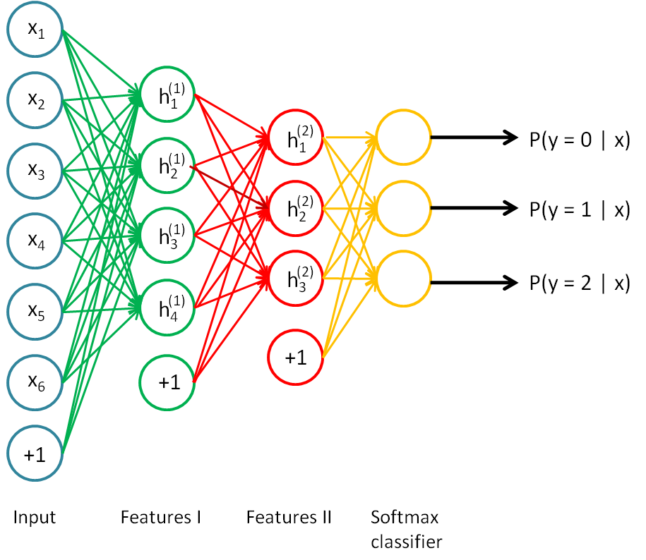
采用贪婪算法,首先把input和feature1看作一个自动编码机,训练出二者之间的参数,然后用feature1层的激活值作为输出,输入到feature2,即把feature1和feature2再看作一个自动编码机,训练出这两层之间的参数,这两步都没有用到分类标签,所以是无监督学习,最后把feature2的激活值作为提取的的特征,输入到分类器,这里需要标签来计算代价函数,从而由优化这个代价函数来训练出feature2与分类器之间的参数,所以这一步是有监督学习,这一步完成之后,把测试样本输入网络,最后会输出该样本分别属于每一类的概率,选出最大概率对应的类别,就是最终的分类结果。
为了使得分类结果更加精确,可以对训练出的参数进行微调,就是在有监督学习之后,我们利用有标签的训练数据可以计算出分类残差,然后利用这个残差反向传播,对已经训练出的参数进行进一步微调,会对最终预测的精度有很大提升
下面是第一层训学习出的特征:

可以看出都是一些笔迹的边缘
作为对比,训练结果显示,微调之后,分类准确度有大幅提升,所以在训练深度网络之后,利用部分标签数据进行微调是一件很有必要的学习:
Before Finetuning Test Accuracy: 91.760%
After Finetuning Test Accuracy: 97.710%
下面是部分程序代码,需要用到,完整代码请先下载minFunc.rar,然后下载stacked_exercise.rar,minFunc.rar里面是lbfgs优化函数,在优化网络参数时需要用到。
%% CS294A/CS294W Stacked Autoencoder Exercise

%  Instructions
%  ------------
%
%  This file contains code that helps you get started on the
%  sstacked autoencoder exercise. You will need to complete code in
%  stackedAECost.m
%  You will also need to have implemented sparseAutoencoderCost.m and
%  softmaxCost.m from previous exercises. You will need the initializeParameters.m
%  loadMNISTImages.m, and loadMNISTLabels.m files from previous exercises.
%
%  For the purpose of completing the assignment, you do not need to
%  change the code in this file.
%
%%======================================================================
%% STEP 0: Here we provide the relevant parameters values that will
%  allow your sparse autoencoder to get good filters; you do not need to
%  change the parameters below.

inputSize = 28 * 28;
numClasses = 10;
hiddenSizeL1 = 200;    % Layer 1 Hidden Size
hiddenSizeL2 = 200;    % Layer 2 Hidden Size
sparsityParam = 0.1;   % desired average activation of the hidden units.
                       % (This was denoted by the Greek alphabet rho, which looks like a lower-case "p",
                       %  in the lecture notes).
lambda = 3e-3;         % weight decay parameter
beta = 3;              % weight of sparsity penalty term

%%======================================================================
%% STEP 1: Load data from the MNIST database
%
%  This loads our training data from the MNIST database files.

% Load MNIST database files
trainData = loadMNISTImages('train-images.idx3-ubyte');
trainLabels = loadMNISTLabels('train-labels.idx1-ubyte');

trainLabels(trainLabels == 0) = 10; % Remap 0 to 10 since our labels need to start from 1

%%======================================================================
%% STEP 2: Train the first sparse autoencoder
%  This trains the first sparse autoencoder on the unlabelled STL training
%  images.
%  If you've correctly implemented sparseAutoencoderCost.m, you don't need
%  to change anything here.


%  Randomly initialize the parameters
sae1Theta = initializeParameters(hiddenSizeL1, inputSize);

%% ---------------------- YOUR CODE HERE  ---------------------------------
%  Instructions: Train the first layer sparse autoencoder, this layer has
%                an hidden size of "hiddenSizeL1"
%                You should store the optimal parameters in sae1OptTheta
addpath minFunc/;
options = struct;
options.Method = 'lbfgs';
options.maxIter = 400;
options.display = 'on';
%训练出第一层网络的参数
[sae1OptTheta, cost] =  minFunc(@(p) sparseAutoencoderCost(p,...
                        inputSize,hiddenSizeL1,lambda,...
                        sparsityParam,beta,trainData),...
                        sae1Theta,options);
save('step2.mat', 'sae1OptTheta');
W1 = reshape(sae1OptTheta(1:hiddenSizeL1 * inputSize), hiddenSizeL1, inputSize);
display_network(W1');
% -------------------------------------------------------------------------

%%======================================================================
%% STEP 2: Train the second sparse autoencoder
%  This trains the second sparse autoencoder on the first autoencoder
%  featurse.
%  If you've correctly implemented sparseAutoencoderCost.m, you don't need
%  to change anything here.

[sae1Features] = feedForwardAutoencoder(sae1OptTheta, hiddenSizeL1, ...
                                        inputSize, trainData);

%  Randomly initialize the parameters
sae2Theta = initializeParameters(hiddenSizeL2, hiddenSizeL1);

%% ---------------------- YOUR CODE HERE  ---------------------------------
%  Instructions: Train the second layer sparse autoencoder, this layer has
%                an hidden size of "hiddenSizeL2" and an inputsize of
%                "hiddenSizeL1"
%
%                You should store the optimal parameters in sae2OptTheta
[sae2OptTheta, cost] =  minFunc(@(p)sparseAutoencoderCost(p,...
                        hiddenSizeL1,hiddenSizeL2,lambda,...
                        sparsityParam,beta,sae1Features),...
                        sae2Theta,options);
% figure;
% W11 = reshape(sae1OptTheta(1:hiddenSizeL1 * inputSize), hiddenSizeL1, inputSize);
% W2 = reshape(sae2OptTheta(1:hiddenSizeL2 * hiddenSizeL1), hiddenSizeL2, hiddenSizeL1);
% figure;
% display_network(W2');
% -------------------------------------------------------------------------


%%======================================================================
%% STEP 3: Train the softmax classifier
%  This trains the sparse autoencoder on the second autoencoder features.
%  If you've correctly implemented softmaxCost.m, you don't need
%  to change anything here.

[sae2Features] = feedForwardAutoencoder(sae2OptTheta, hiddenSizeL2, ...
                                        hiddenSizeL1, sae1Features);

%  Randomly initialize the parameters
saeSoftmaxTheta = 0.005 * randn(hiddenSizeL2 * numClasses, 1);


%% ---------------------- YOUR CODE HERE  ---------------------------------
%  Instructions: Train the softmax classifier, the classifier takes in
%                input of dimension "hiddenSizeL2" corresponding to the
%                hidden layer size of the 2nd layer.
%
%                You should store the optimal parameters in saeSoftmaxOptTheta
%
%  NOTE: If you used softmaxTrain to complete this part of the exercise,
%        set saeSoftmaxOptTheta = softmaxModel.optTheta(:);
softmaxLambda = 1e-4;
numClasses = 10;
softoptions = struct;
softoptions.maxIter = 400;
softmaxModel = softmaxTrain(hiddenSizeL2,numClasses,softmaxLambda,...
                            sae2Features,trainLabels,softoptions);
saeSoftmaxOptTheta = softmaxModel.optTheta(:);

save('step4.mat', 'saeSoftmaxOptTheta');


% -------------------------------------------------------------------------


%%======================================================================
%% STEP 5: Finetune softmax model

% Implement the stackedAECost to give the combined cost of the whole model
% then run this cell.

% Initialize the stack using the parameters learned
stack = cell(2,1);
stack{1}.w = reshape(sae1OptTheta(1:hiddenSizeL1*inputSize), ...
                     hiddenSizeL1, inputSize);
stack{1}.b = sae1OptTheta(2*hiddenSizeL1*inputSize+1:2*hiddenSizeL1*inputSize+hiddenSizeL1);
stack{2}.w = reshape(sae2OptTheta(1:hiddenSizeL2*hiddenSizeL1), ...
                     hiddenSizeL2, hiddenSizeL1);
stack{2}.b = sae2OptTheta(2*hiddenSizeL2*hiddenSizeL1+1:2*hiddenSizeL2*hiddenSizeL1+hiddenSizeL2);

% Initialize the parameters for the deep model
[stackparams, netconfig] = stack2params(stack);
stackedAETheta = [ saeSoftmaxOptTheta ; stackparams ];

%% ---------------------- YOUR CODE HERE  ---------------------------------
%  Instructions: Train the deep network, hidden size here refers to the '
%                dimension of the input to the classifier, which corresponds
%                to "hiddenSizeL2".
%
%
[stackedAEOptTheta, cost] =  minFunc(@(p)stackedAECost(p,inputSize,hiddenSizeL2,...
                         numClasses, netconfig,lambda, trainData, trainLabels),...
                        stackedAETheta,options);
save('step5.mat', 'stackedAEOptTheta');
% -------------------------------------------------------------------------


%%======================================================================
%% STEP 6: Test
%  Instructions: You will need to complete the code in stackedAEPredict.m
%                before running this part of the code
%

% Get labelled test images
% Note that we apply the same kind of preprocessing as the training set
testData = loadMNISTImages('t10k-images.idx3-ubyte');
testLabels = loadMNISTLabels('t10k-labels.idx1-ubyte');

testLabels(testLabels == 0) = 10; % Remap 0 to 10

[pred] = stackedAEPredict(stackedAETheta, inputSize, hiddenSizeL2, ...
                          numClasses, netconfig, testData);

acc = mean(testLabels(:) == pred(:));
fprintf('Before Finetuning Test Accuracy: %0.3f%%
', acc * 100);

[pred] = stackedAEPredict(stackedAEOptTheta, inputSize, hiddenSizeL2, ...
                          numClasses, netconfig, testData);

acc = mean(testLabels(:) == pred(:));
fprintf('After Finetuning Test Accuracy: %0.3f%%
', acc * 100);

% Accuracy is the proportion of correctly classified images
% The results for our implementation were:
%
% Before Finetuning Test Accuracy: 87.7%
% After Finetuning Test Accuracy:  97.6%
%
% If your values are too low (accuracy less than 95%), you should check
% your code for errors, and make sure you are training on the
% entire data set of 60000 28x28 training images
% (unless you modified the loading code, this should be the case)
function [ cost, grad ] = stackedAECost(theta, inputSize, hiddenSize, ...
                                              numClasses, netconfig, ...
                                              lambda, data, labels)

% stackedAECost: Takes a trained softmaxTheta and a training data set with labels,
% and returns cost and gradient using a stacked autoencoder model. Used for
% finetuning.

% theta: trained weights from the autoencoder
% visibleSize: the number of input units
% hiddenSize:  the number of hidden units *at the 2nd layer*
% numClasses:  the number of categories
% netconfig:   the network configuration of the stack
% lambda:      the weight regularization penalty
% data: Our matrix containing the training data as columns.  So, data(:,i) is the i-th training example.
% labels: A vector containing labels, where labels(i) is the label for the
% i-th training example


%% Unroll softmaxTheta parameter

% We first extract the part which compute the softmax gradient
softmaxTheta = reshape(theta(1:hiddenSize*numClasses), numClasses, hiddenSize);

% Extract out the "stack"
stack = params2stack(theta(hiddenSize*numClasses+1:end), netconfig);

% You will need to compute the following gradients
softmaxThetaGrad = zeros(size(softmaxTheta));
stackgrad = cell(size(stack));
for d = 1:numel(stack)
    stackgrad{d}.w = zeros(size(stack{d}.w));
    stackgrad{d}.b = zeros(size(stack{d}.b));
end

cost = 0; % You need to compute this

% You might find these variables useful
M = size(data, 2);
groundTruth = full(sparse(labels, 1:M, 1));


%% --------------------------- YOUR CODE HERE -----------------------------
%  Instructions: Compute the cost function and gradient vector for
%                the stacked autoencoder.
%
%                You are given a stack variable which is a cell-array of
%                the weights and biases for every layer. In particular, you
%                can refer to the weights of Layer d, using stack{d}.w and
%                the biases using stack{d}.b . To get the total number of
%                layers, you can use numel(stack).
%
%                The last layer of the network is connected to the softmax
%                classification layer, softmaxTheta.
%
%                You should compute the gradients for the softmaxTheta,
%                storing that in softmaxThetaGrad. Similarly, you should
%                compute the gradients for each layer in the stack, storing
%                the gradients in stackgrad{d}.w and stackgrad{d}.b
%                Note that the size of the matrices in stackgrad should
%                match exactly that of the size of the matrices in stack.
%

depth = numel(stack);
z = cell(depth+1,1);
a = cell(depth+1, 1);
a{1} = data;

for layer = (1:depth)
  z{layer+1} = stack{layer}.w * a{layer} + repmat(stack{layer}.b, [1, size(a{layer},2)]);
  a{layer+1} = sigmoid(z{layer+1});
end

M = softmaxTheta * a{depth+1};
M = bsxfun(@minus, M, max(M));
p = bsxfun(@rdivide, exp(M), sum(exp(M)));

cost = -1/numClasses * groundTruth(:)' * log(p(:)) + lambda/2 * sum(softmaxTheta(:) .^ 2);
softmaxThetaGrad = -1/numClasses * (groundTruth - p) * a{depth+1}' + lambda * softmaxTheta;

d = cell(depth+1);

d{depth+1} = -(softmaxTheta' * (groundTruth - p)) .* a{depth+1} .* (1-a{depth+1});

for layer = (depth:-1:2)
  d{layer} = (stack{layer}.w' * d{layer+1}) .* a{layer} .* (1-a{layer});
end

for layer = (depth:-1:1)
  stackgrad{layer}.w = (1/numClasses) * d{layer+1} * a{layer}';
  stackgrad{layer}.b = (1/numClasses) * sum(d{layer+1}, 2);
end
% -------------------------------------------------------------------------

%% Roll gradient vector
grad = [softmaxThetaGrad(:) ; stack2params(stackgrad)];

end


% You might find this useful
function sigm = sigmoid(x)
    sigm = 1 ./ (1 + exp(-x));
end
function [pred] = stackedAEPredict(theta, inputSize, hiddenSize, numClasses, netconfig, data)

% stackedAEPredict: Takes a trained theta and a test data set,
% and returns the predicted labels for each example.

% theta: trained weights from the autoencoder
% visibleSize: the number of input units
% hiddenSize:  the number of hidden units *at the 2nd layer*
% numClasses:  the number of categories
% data: Our matrix containing the training data as columns.  So, data(:,i) is the i-th training example.

% Your code should produce the prediction matrix
% pred, where pred(i) is argmax_c P(y(c) | x(i)).

%% Unroll theta parameter

% We first extract the part which compute the softmax gradient
softmaxTheta = reshape(theta(1:hiddenSize*numClasses), numClasses, hiddenSize);

% Extract out the "stack"
stack = params2stack(theta(hiddenSize*numClasses+1:end), netconfig);

%% ---------- YOUR CODE HERE --------------------------------------
%  Instructions: Compute pred using theta assuming that the labels start
%                from 1.

depth = numel(stack);
z = cell(depth+1,1);
a = cell(depth+1, 1);
a{1} = data;

for layer = (1:depth)
  z{layer+1} = stack{layer}.w * a{layer} + repmat(stack{layer}.b, [1, size(a{layer},2)]);
  a{layer+1} = sigmoid(z{layer+1});
end

[~, pred] = max(softmaxTheta * a{depth+1});


% -----------------------------------------------------------

end


% You might find this useful
function sigm = sigmoid(x)
    sigm = 1 ./ (1 + exp(-x));
end