逻辑回归从零开始实现

1 导入实验需要的包

import torch
import matplotlib.pyplot as plt
import numpy as np
import os
os.environ["KMP_DUPLICATE_LIB_OK"]  =  "TRUE"

 

2 人工构造数据集

　　生成正/负样本各 50 个，特征数为 2，进行二分类（0、1）.

n_data = torch.ones(50, 2)  
x1 = torch.normal(2 * n_data, 1)  
y1 = torch.zeros(50) 

x2 = torch.normal(-2 * n_data, 1)  
y2 = torch.ones(50)  

x = torch.cat((x1, x2), 0).type(torch.FloatTensor)
y = torch.cat((y1, y2), 0).type(torch.FloatTensor)

datax = x.numpy()

3 绘制数据散点图

fig,ax = plt.subplots()
#第 一 类样本
ax.scatter(x.numpy()[:50, 0], x.numpy()[:50, 1], s=35, c='b', marker='o', label='class 0')
#第 二 类样本
ax.scatter(x.numpy()[50:, 0], x.numpy()[50:, 1], s=35, c='r', marker='x', label='class 1')

ax.legend()
plt.show()

　　　　　　

4  初始化模型参数

　　设置 $theta=[w_0,w_1,w_2]$ 初始化为 1  ，学习率 $alpha=0.004$，迭代次数 $iters =20000$ ，其中 $w_0$ 代表偏置 $b$

theta = np.zeros((3,1))
alpha = 0.004
iters = 20000
Train_Loss_list = []

5 定义模型

#设置sigmoid函数，通过传进去的值算出概率，通过概率来做出判断
def sigmoid(inX):                       #inX指的是wT*x，这里的w和x都是向量
    return 1.0 / (1 + np.exp(-inX))

6 定义损失函数

　　损失函数使用交叉熵损失

# 实现逻辑回归的代价函数，两个部分，-y(log(hx)和-(1-y)log(1-hx)
def cost_Func(theta, X, y):
    A = sigmoid(X@theta)
    first = y*np.log(A)
    second = (1-y)*np.log(1-A)
    return -np.sum(first+second)/len(X)

7 定义优化算法

　　采用随机梯度下降法，更新参数

def gradientDescent (X,y,theta,iters,alpha):
    global Train_Loss_list
    m = len(X)
    for i in range(iters+1):
        A=sigmoid(X@theta)
        theta = theta-(alpha/m)*X.T@(A-y)
        cost =cost_Func(theta,X,y)
        Train_Loss_list.append(cost)
        if i % 1000==0:
            print("第"+str(i)+" 次的损失为 "+str(cost))
    print(len(Train_Loss_list))
    return theta

8 训练模型

　　获得训练 20000次 中的损失变化，以及最终的权重和偏置。

x = x.numpy()
#增加一列全为 1 ，方便与偏置项相乘。
ones = np.ones(100)

x = np.c_[ones,x]
y = y.numpy().reshape(100,1)

theta = np.zeros((3,1))
#print("theta.shape=",theta.shape)

theta_final = gradientDescent(x,y,theta,iters,alpha)

#得到最终的 权重和偏置。
print("theta_final=[",theta_final[0][0],theta_final[1][0],theta_final[2][0]," ]")

9 绘制训练损失图

x11= range(0,20001)
y11= Train_Loss_list
plt.xlabel('Train loss vs. epoches')
plt.ylabel('Train loss')
plt.plot(x11, y11,'.',c='b',label="Train_Loss")
plt.legend()
plt.show()

10 预测函数定义

def predict(X,theta):
    prob = sigmoid(X@theta)
    return [1 if x>=0.5 else 0 for x in prob]

　　使用预测函数获取原始数据集的准确率

y_ = np.array(predict(x,theta_final))
y_pre = y_.reshape(len(y_),1 )
acc = np.mean(y_pre == y)
print(acc)

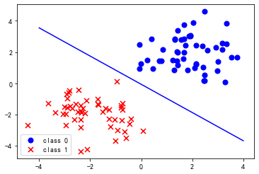
11 结果可视化

　　使用一条直线将两类数据区分开来。

coef1 = -theta_final[0,0] / theta_final[2,0]
coef2 = -theta_final[1,0] / theta_final[2,0]
x1 = np.linspace(-4,4,100)
f = coef1+coef2*x1


fig,ax = plt.subplots()
ax.plot(x1,f,c='blue')
ax.scatter(datax[:50, 0],datax[:50, 1], s=50, c='b', marker='o', label='class 0')
ax.scatter(datax[50:, 0], datax[50:, 1], s=50, c='r', marker='x', label='class 1')
ax.legend()
plt.show()