pandas深入理解

Pandas是一个Python库，旨在通过“标记”和“关系”数据以完成数据整理工作，库中有两个主要的数据结构Series和DataFrame

In [1]: import numpy as np
In [2]: import pandas as pd
In [3]: from pandas import Series,DataFrame
In [4]: import matplotlib.pyplot as plt

本文主要说明完成数据整理的几大步骤：

1.数据来源

1）加载数据

2）随机采样

2.数据清洗

0）数据统计（贯穿整个过程）

1）处理缺失值

2）层次化索引

3）类数据库操作（增、删、改、查、连接）

4）离散面元划分

5）重命名轴索引

3.数据转换

1）分组

2）聚合

3）数据可视化

数据来源

1.加载数据

pandas提供了一些将表格型数据读取为DataFrame对象的函数，其中用的比较多的是read_csv和read_table，参数说明如下：

参数	说明
path	表示文件位置、URL、文件型对象的字符串
sep或delimiter	用于将行中的各字段进行拆分的字符串或正则表达式
head	用作列名的行号
index_col	用作行索引的列编号或列名
skiprows	需要跳过的行号列表（从0开始）
na_value	一组用户替换的值
converters	由列号/列名跟函数之间的映射关系组成的字典
chunksize	文件快的大小

举例：

In [2]:  result = pd.read_table('C:UsersHPDesktopSEC-DEBIT_0804.txt',sep = 's+')

In [3]: result
Out[3]:
          SEC-DEBIT HKD0002481145000001320170227SECURITIES  BUY  ON  23Feb2017
0    10011142009679                HKD00002192568083002000  NaN NaN        NaN
1    20011142009679                HKD00004154719083002000  NaN NaN        NaN
2    30011142005538                HKD00000210215083002300  NaN NaN        NaN
3    40011142005538                HKD00000140211083002300  NaN NaN        NaN

延展：

DataFrame写文件：data.to_csv('*.csv')

Series写文件：data.to_csv('*.csv')

Series读文件：Series.from_csv('*.csv')

2.随机采样

利用numpy.random.permutation函数可以实现对Series和DataFrame的列随机重排序工作

In [18]: df = DataFrame(np.arange(20).reshape(5,4))
In [19]: df
Out[19]:
    0   1   2   3
0   0   1   2   3
1   4   5   6   7
2   8   9  10  11
3  12  13  14  15
4  16  17  18  19

In [20]: sample = np.random.permutation(5)
In [21]: sample
Out[21]: array([0, 1, 4, 2, 3])

In [22]: df.take(sample)
Out[22]:
    0   1   2   3
0   0   1   2   3
1   4   5   6   7
4  16  17  18  19
2   8   9  10  11
3  12  13  14  15

In [25]:  df.take(np.random.permutation(5)[:3])
Out[25]:
    0   1   2   3
2   8   9  10  11
4  16  17  18  19
3  12  13  14  15

数据清洗

0.数据统计

In [31]: df = DataFrame({'A':np.random.randn(5),'B':np.random.randn(5)})

In [32]: df
Out[32]:
          A         B
0 -0.635732  0.738902
1 -1.100320  0.910203
2  1.503987 -2.030411
3  0.548760  0.228552
4 -2.201917  1.676173

In [33]: df.count()    #计算个数
Out[33]:
A    5
B    5
dtype: int64
In [34]: df.min()   #最小值
Out[34]:
A   -2.201917
B   -2.030411
dtype: float64
In [35]: df.max()   #最大值
Out[35]:
A    1.503987
B    1.676173
dtype: float64
In [36]: df.idxmin()  #最小值的位置
Out[36]:
A    4
B    2
dtype: int64
In [37]: df.idxmax()   #最大值的位置
Out[37]:
A    2
B    4
dtype: int64
In [38]: df.sum()    #求和
Out[38]:
A   -1.885221
B    1.523419
dtype: float64
In [39]: df.mean()   #平均数
Out[39]:
A   -0.377044
B    0.304684
dtype: float64
In [40]: df.median()   #中位数
Out[40]:
A   -0.635732
B    0.738902
dtype: float64
In [41]: df.mode()  #众数
Out[41]:
Empty DataFrame
Columns: [A, B]
Index: []
In [42]: df.var()    #方差
Out[42]:
A    2.078900
B    1.973661
dtype: float64
In [43]: df.std()    #标准差
Out[43]:
A    1.441839
B    1.404871
dtype: float64
In [44]: df.mad()    #平均绝对偏差
Out[44]:
A    1.122734
B    0.964491
dtype: float64
In [45]: df.skew()   #偏度
Out[45]:
A    0.135719
B   -1.480080
dtype: float64
In [46]: df.kurt()   #峰度
Out[46]:
A   -0.878539
B    2.730675
dtype: float64
In [48]: df.quantile(0.25)   #25%分位数
Out[48]:
A   -1.100320
B    0.228552
dtype: float64
In [49]: df.describe()    #描述性统计指标
Out[49]:
              A         B
count  5.000000  5.000000
mean  -0.377044  0.304684
std    1.441839  1.404871
min   -2.201917 -2.030411
25%   -1.100320  0.228552
50%   -0.635732  0.738902
75%    0.548760  0.910203
max    1.503987  1.676173

1.处理缺失值

In [50]: string = Series(['apple','banana','pear',np.nan,'grape'])

In [51]: string
Out[51]:
0     apple
1    banana
2      pear
3       NaN
4     grape
dtype: object

In [52]: string.isnull()  #判断是否为缺失值
Out[52]:
0    False
1    False
2    False
3     True
4    False
dtype: bool

In [53]: string.dropna()  #过滤缺失值，默认过滤任何含NaN的行
Out[53]:
0     apple
1    banana
2      pear
4     grape
dtype: object

In [54]: string.fillna(0)  #填充缺失值
Out[54]:
0     apple
1    banana
2      pear
3         0
4     grape
dtype: object

In [55]: string.ffill()   #向前填充
Out[55]:
0     apple
1    banana
2      pear
3      pear
4     grape
dtype: object

In [56]: data = DataFrame([[1. ,6.5,3],[1. ,np.nan,np.nan],[np.nan,np.nan,np.nan],[np.nan,7,9]])  #DataFrame操作同理
In [57]: data
Out[57]:
     0    1    2
0  1.0  6.5  3.0
1  1.0  NaN  NaN
2  NaN  NaN  NaN
3  NaN  7.0  9.0

2.层次化索引

In [6]:  data = Series(np.random.randn(10),index=[['a','a','a','b','b','b','c','c','d','d'],[1,2,3,1,2,3,1,2,2,3]])

In [7]: data
Out[7]:
a  1    0.386697
   2    0.822063
   3    0.338441
b  1    0.017249
   2    0.880122
   3    0.296465
c  1    0.376104
   2   -1.309419
d  2    0.512754
   3    0.223535
dtype: float64

In [8]: data.index  
Out[8]:
MultiIndex(levels=[[u'a', u'b', u'c', u'd'], [1, 2, 3]],
           labels=[[0, 0, 0, 1, 1, 1, 2, 2, 3, 3], [0, 1, 2, 0, 1, 2, 0, 1, 1, 2]])


In [10]: data['b':'c']
Out[10]:
b  1    0.017249
   2    0.880122
   3    0.296465
c  1    0.376104
   2   -1.309419
dtype: float64

In [11]: data[:,2]
Out[11]:
a    0.822063
b    0.880122
c   -1.309419
d    0.512754
dtype: float64

In [12]: data.unstack()
Out[12]:
          1         2         3
a  0.386697  0.822063  0.338441
b  0.017249  0.880122  0.296465
c  0.376104 -1.309419       NaN
d       NaN  0.512754  0.223535

In [13]: data.unstack().stack()
Out[13]:
a  1    0.386697
   2    0.822063
   3    0.338441
b  1    0.017249
   2    0.880122
   3    0.296465
c  1    0.376104
   2   -1.309419
d  2    0.512754
   3    0.223535
dtype: float64

In [14]: df = DataFrame(np.arange(12).reshape(4,3),index=[['a','a','b','b'],[1,2,1,2]],columns=[['Ohio','Ohio','Colorad
    ...: o'],['Green','Red','Green']])

In [15]: df
Out[15]:
     Ohio     Colorado
    Green Red    Green
a 1     0   1        2
  2     3   4        5
b 1     6   7        8
  2     9  10       11

In [16]: df.index.names = ['key1','key2']
In [17]: df.columns.names = ['state','color']

In [18]: df
Out[18]:
state      Ohio     Colorado
color     Green Red    Green
key1 key2
a    1        0   1        2
     2        3   4        5
b    1        6   7        8
     2        9  10       11

In [19]: df['Ohio']    #降维
Out[19]:
color      Green  Red
key1 key2
a    1         0    1
     2         3    4
b    1         6    7
     2         9   10

In [20]: df.swaplevel('key1','key2')
Out[20]:
state      Ohio     Colorado
color     Green Red    Green
key2 key1
1    a        0   1        2
2    a        3   4        5
1    b        6   7        8
2    b        9  10       11

In [21]: df.sortlevel(1)    #key2
Out[21]:
state      Ohio     Colorado
color     Green Red    Green
key1 key2
a    1        0   1        2
b    1        6   7        8
a    2        3   4        5
b    2        9  10       11

In [22]: df.sortlevel(0)  #key1
Out[22]:
state      Ohio     Colorado
color     Green Red    Green
key1 key2
a    1        0   1        2
     2        3   4        5
b    1        6   7        8
     2        9  10       11

3.类sql操作

In [5]: dic = {'Name':['LiuShunxiang','Zhangshan','ryan'],
   ...: 'Sex':['M','F','F'],
   ...: 'Age':[27,23,24],
   ...: 'Height':[165.7,167.2,154],
   ...: 'Weight':[61,63,41]}

In [6]: student = pd.DataFrame(dic)
In [7]: student
Out[7]:
   Age  Height          Name Sex  Weight
0   27   165.7  LiuShunxiang   M      61
1   23   167.2     Zhangshan   F      63
2   24   154.0          ryan   F      41

In [8]: dic1 = {'Name':['Ann','Joe'],
   ...: 'Sex':['M','F'],
   ...: 'Age':[27,33],
   ...: 'Height':[168,177.2],
   ...: 'Weight':[51,65]}

In [9]: student1 =  pd.DataFrame(dic1)

In [10]: Student = pd.concat([student,student1])  #插入行
In [11]: Student
Out[11]:
   Age  Height          Name Sex  Weight
0   27   165.7  LiuShunxiang   M      61
1   23   167.2     Zhangshan   F      63
2   24   154.0          ryan   F      41
0   27   168.0           Ann   M      51
1   33   177.2           Joe   F      65

In [14]:  pd.DataFrame(Student,columns = ['Age','Height','Name','Sex','Weight','Score'])   #新增列
Out[14]:
   Age  Height          Name Sex  Weight  Score
0   27   165.7  LiuShunxiang   M      61    NaN
1   23   167.2     Zhangshan   F      63    NaN
2   24   154.0          ryan   F      41    NaN
0   27   168.0           Ann   M      51    NaN
1   33   177.2           Joe   F      65    NaN

In [16]:  Student.ix[Student['Name']=='ryan','Height'] = 160  #修改某个数据
In [17]: Student
Out[17]:
   Age  Height          Name Sex  Weight
0   27   165.7  LiuShunxiang   M      61
1   23   167.2     Zhangshan   F      63
2   24   160.0          ryan   F      41
0   27   168.0           Ann   M      51
1   33   177.2           Joe   F      65

In [18]: Student[Student['Height']>160]   #删选
Out[18]:
   Age  Height          Name Sex  Weight
0   27   165.7  LiuShunxiang   M      61
1   23   167.2     Zhangshan   F      63
0   27   168.0           Ann   M      51
1   33   177.2           Joe   F      65

In [21]: Student.drop(['Weight'],axis = 1).head() #删除列
Out[21]:
   Age  Height          Name Sex
0   27   165.7  LiuShunxiang   M
1   23   167.2     Zhangshan   F
2   24   160.0          ryan   F
0   27   168.0           Ann   M
1   33   177.2           Joe   F

In [22]: Student.drop([1,2])   #删除行索引为1和2的行
Out[22]:
   Age  Height          Name Sex  Weight
0   27   165.7  LiuShunxiang   M      61
0   27   168.0           Ann   M      51

In [24]: Student.drop(['Age'],axis = 1)   #删除列索引为Age的列
Out[24]:
   Height          Name Sex  Weight
0   165.7  LiuShunxiang   M      61
1   167.2     Zhangshan   F      63
2   154.0          ryan   F      41
0   168.0           Ann   M      51
1   177.2           Joe   F      65


In [26]: Student.groupby('Sex').agg([np.mean,np.median])   #等价于SELECT…FROM…GROUP BY…功能
Out[26]:
           Age             Height             Weight
          mean median        mean  median       mean median
Sex
F    26.666667     24  168.133333  167.20  56.333333     63
M    27.000000     27  166.850000  166.85  56.000000     56

In [27]: series = pd.Series(np.random.randint(1,20,5))    #排序
In [28]: series
Out[28]:
0     9
1    17
2    17
3    13
4    15
dtype: int32

In [29]: series.order()   #默认升序
C:/Anaconda2/Scripts/ipython-script.py:1: FutureWarning: order is deprecated, use sort_values(...)
  if __name__ == '__main__':
Out[29]:
0     9
3    13
4    15
1    17
2    17
dtype: int32

In [30]: series.order(ascending = False)  #降序
C:/Anaconda2/Scripts/ipython-script.py:1: FutureWarning: order is deprecated, use sort_values(...)
  if __name__ == '__main__':
Out[30]:
2    17
1    17
4    15
3    13
0     9
dtype: int32

In [31]: Student.sort_values(by = ['Height'])   #按值排序
Out[31]:
   Age  Height          Name Sex  Weight
2   24   160.0          ryan   F      41
0   27   165.7  LiuShunxiang   M      61
1   23   167.2     Zhangshan   F      63
0   27   168.0           Ann   M      51
1   33   177.2           Joe   F      65

In [32]: dict2 = {'Name':['ryan','LiuShunxiang','Zhangshan','Ann','Joe'],   
    ...:          'Score':['89','90','78','60','53']}

In [33]: Score = pd.DataFrame(dict2)
In [34]: Score
Out[34]:
           Name Score
0          ryan    89
1  LiuShunxiang    90
2     Zhangshan    78
3           Ann    60
4           Joe    53

In [35]: stu_score = pd.merge(Student,Score,on = 'Name')   #表连接
In [36]: stu_score
Out[36]:
   Age  Height          Name Sex  Weight Score
0   27   165.7  LiuShunxiang   M      61    90
1   23   167.2     Zhangshan   F      63    78
2   24   160.0          ryan   F      41    89
3   27   168.0           Ann   M      51    60
4   33   177.2           Joe   F      65    53 

注：student1以dic形式转DataFrame对象和直接新建DataFrame对象，连接结果不同

In [71]:student1 =  DataFrame({'name';['Ann','Joe'],'Sex':['M','F'],'Age':[27,33],'Height':[168,177.2],'Weight':[51,65
    ...: ]})
In [72]: student
Out[72]:
   Age  Height          Name Sex  Weight
0   27   165.7  LiuShunxiang   M      61
1   23   167.2     Zhangshan   F      63
2   24   154.0          ryan   F      41

In [73]: student1
Out[73]:
   Age  Height Sex  Weight name
0   27   168.0   M      51  Ann
1   33   177.2   F      65  Joe

In [74]: Student = pd.concat([student,student1])
In [75]: Student
Out[75]:
   Age  Height          Name Sex  Weight name
0   27   165.7  LiuShunxiang   M      61  NaN
1   23   167.2     Zhangshan   F      63  NaN
2   24   154.0          ryan   F      41  NaN
0   27   168.0           NaN   M      51  Ann
1   33   177.2           NaN   F      65  Joe

延伸表连接，merge函数参数说明如下：

参数	说明
left	参与合并的左侧DataFrame
right	参与合并的右侧DataFrame
how	"inner"、"outer"、"left"、"right"其中之一，默认为inner
on	用于连接的列名
left_on	左侧DataFrame中用作连接键的列
right_on	右侧DataFrame中用作连接键的列
left_index	将左侧DataFrame中的行索引作为连接的键
right_index	将右侧DataFrame中的行索引作为连接的键
sort	根据连接键对合并后的数据进行排序

 举例如下

In [5]:  df1 = DataFrame({'key':['b','b','a','c','a','a','b'],'data1':range(7)})
In [6]: df1
Out[6]:
   data1 key
0      0   b
1      1   b
2      2   a
3      3   c
4      4   a
5      5   a
6      6   b

In [7]: df2 = DataFrame({'key':['a','b','d'],'data2':range(3)})
In [8]: df2
Out[8]:
   data2 key
0      0   a
1      1   b
2      2   d

In [9]: pd.merge(df1,df2)   #默认内链接，合并相同的key即a,b
Out[9]:
   data1 key  data2
0      0   b      1
1      1   b      1
2      6   b      1
3      2   a      0
4      4   a      0
5      5   a      0

In [10]: df3 = DataFrame({'lkey':['b','b','a','c','a','a','b'],'data1':range(7)})
In [11]: df4 = DataFrame({'rkey':['a','b','d'],'data2':range(3)})

In [12]: df3
Out[12]:
   data1 lkey
0      0    b
1      1    b
2      2    a
3      3    c
4      4    a
5      5    a
6      6    b

In [13]: df4
Out[13]:
   data2 rkey
0      0    a
1      1    b
2      2    d

In [14]: print pd.merge(df3,df4,left_on = 'lkey',right_on = 'rkey')
   data1 lkey  data2 rkey
0      0    b      1    b
1      1    b      1    b
2      6    b      1    b
3      2    a      0    a
4      4    a      0    a
5      5    a      0    a

In [15]: print pd.merge(df3,df4,left_on = 'lkey',right_on = 'data2')
Empty DataFrame
Columns: [data1, lkey, data2, rkey]
Index: []

In [16]: print pd.merge(df1,df2,how = 'outer')
   data1 key  data2
0    0.0   b    1.0
1    1.0   b    1.0
2    6.0   b    1.0
3    2.0   a    0.0
4    4.0   a    0.0
5    5.0   a    0.0
6    3.0   c    NaN
7    NaN   d    2.0

In [17]: df5 = DataFrame({'key':list('bbacab'),'data1':range(6)})
In [18]: df6 = DataFrame({'key':list('ababd'),'data2':range(5)})
In [19]: df5
Out[19]:
   data1 key
0      0   b
1      1   b
2      2   a
3      3   c
4      4   a
5      5   b

In [20]: df6
Out[20]:
   data2 key
0      0   a
1      1   b
2      2   a
3      3   b
4      4   d

In [21]: print pd.merge(df5,df6,on = 'key',how = 'left')
    data1 key  data2
0       0   b    1.0
1       0   b    3.0
2       1   b    1.0
3       1   b    3.0
4       2   a    0.0
5       2   a    2.0
6       3   c    NaN
7       4   a    0.0
8       4   a    2.0
9       5   b    1.0
10      5   b    3.0

In [22]: left = DataFrame({'key1':['foo','foo','bar'],'key2':['one','two','one'],'lval':[1,2,3]})
In [23]: right = DataFrame({'key1':['foo','foo','bar','bar'],'key2':['one','one','one','two'],'rval':[4,5,6,7]})
In [24]: left
Out[24]:
  key1 key2  lval
0  foo  one     1
1  foo  two     2
2  bar  one     3

In [25]: right
Out[25]:
  key1 key2  rval
0  foo  one     4
1  foo  one     5
2  bar  one     6
3  bar  two     7

In [26]: print pd.merge(left,right,on = ['key1','key2'],how = 'outer')
  key1 key2  lval  rval
0  foo  one   1.0   4.0
1  foo  one   1.0   5.0
2  foo  two   2.0   NaN
3  bar  one   3.0   6.0
4  bar  two   NaN   7.0

In [27]: print pd.merge(left,right,on = 'key1')
  key1 key2_x  lval key2_y  rval
0  foo    one     1    one     4
1  foo    one     1    one     5
2  foo    two     2    one     4
3  foo    two     2    one     5
4  bar    one     3    one     6
5  bar    one     3    two     7

In [28]: print pd.merge(left,right,on = 'key1',suffixes = ('_left','_right'))
  key1 key2_left  lval key2_right  rval
0  foo       one     1        one     4
1  foo       one     1        one     5
2  foo       two     2        one     4
3  foo       two     2        one     5
4  bar       one     3        one     6
5  bar       one     3        two     7

4.离散化面元划分

In [17]: age = [20,22,25,27,21,23,37,31,61,45,41,32]
In [18]: bins = [18,25,35,60,100]

In [19]: cats = pd.cut(age,bins)
In [20]: cats
Out[20]:
[(18, 25], (18, 25], (18, 25], (25, 35], (18, 25], ..., (25, 35], (60, 100], (35, 60], (35, 60], (25, 35]]
Length: 12
Categories (4, object): [(18, 25] < (25, 35] < (35, 60] < (60, 100]]

In [26]:  group_names = ['YoungAdult','Adult','MiddleAged','Senior']

In [27]: pd.cut(age,bins,labels = group_names)  #设置面元名称
Out[27]:
[YoungAdult, YoungAdult, YoungAdult, Adult, YoungAdult, ..., Adult, Senior, MiddleAged, MiddleAged, Adult]
Length: 12
Categories (4, object): [YoungAdult < Adult < MiddleAged < Senior]

In [28]: data = np.random.randn(10)

In [29]: cats = pd.qcut(data,4)   #qcut提供根据样本分位数对数据进行面元划分
In [30]: cats
Out[30]:
[(0.268, 0.834], (-0.115, 0.268], (0.268, 0.834], [-1.218, -0.562], (-0.562, -0.115], [-1.218, -0.562], (-0.115, 0.268], [-1.218, -0.562], (0.268, 0.834], (-0.562, -0.115]]
Categories (4, object): [[-1.218, -0.562] < (-0.562, -0.115] < (-0.115, 0.268] < (0.268, 0.834]]


In [33]: pd.value_counts(cats)
Out[33]:
(0.268, 0.834]      3
[-1.218, -0.562]    3
(-0.115, 0.268]     2
(-0.562, -0.115]    2
dtype: int64

In [35]:  pd.qcut(data,[0.1,0.5,0.9,1.])  #自定义分位数，[0-1]的数值
Out[35]:
[(-0.115, 0.432], (-0.115, 0.432], (0.432, 0.834], NaN, [-0.787, -0.115], [-0.787, -0.115], (-0.115, 0.432], [-0.787, -0.115], (-0.115, 0.432], [-0.787, -0.115]]
Categories (3, object): [[-0.787, -0.115] < (-0.115, 0.432] < (0.432, 0.834]]

5.重命名轴索引

In [36]: data = DataFrame(np.arange(12).reshape(3,4),index = ['Ohio','Colorado','New York'],columns = ['one','two','thr
    ...: ee','four'])

In [37]: data
Out[37]:
          one  two  three  four
Ohio        0    1      2     3
Colorado    4    5      6     7
New York    8    9     10    11

In [38]: data.index = data.index.map(str.upper)
In [39]: data
Out[39]:
          one  two  three  four
OHIO        0    1      2     3
COLORADO    4    5      6     7
NEW YORK    8    9     10    11

In [40]: data.rename(index = str.title,columns=str.upper)
Out[40]:
          ONE  TWO  THREE  FOUR
Ohio        0    1      2     3
Colorado    4    5      6     7
New York    8    9     10    11

In [41]: data.rename(index={'OHIO':'INDIANA'},columns={'three':'ryana'})  #对部分轴标签更新
Out[41]:
          one  two  ryana  four
INDIANA     0    1      2     3
COLORADO    4    5      6     7
NEW YORK    8    9     10    11

数据转换

1.分组

In [42]: df = DataFrame({'key1':['a','a','b','b','a'],'key2':['one','two','one','two','one'],'data1':np.random.randn(5)
    ...: ,'data2':np.random.randn(5)})

In [43]: df
Out[43]:
      data1     data2 key1 key2
0  0.762448  0.816634    a  one
1  1.412613  0.867923    a  two
2  0.899297 -1.049657    b  one
3  0.912080  0.628012    b  two
4 -0.549258 -1.327614    a  one

In [44]: grouped = df['data1'].groupby(df['key1'])    #按key1列分组，计算data1列的平均值
In [45]: grouped
Out[45]: <pandas.core.groupby.SeriesGroupBy object at 0x00000000073C97F0>

In [46]: grouped.mean()
Out[46]:
key1
a    0.541935
b    0.905688
Name: data1, dtype: float64


In [48]: df['data1'].groupby([df['key1'],df['key2']]).mean()
Out[48]:
key1  key2
a     one     0.106595
      two     1.412613
b     one     0.899297
      two     0.912080
Name: data1, dtype: float64

In [49]: df.groupby('key1').mean()    #根据列名分组
Out[49]:
         data1     data2
key1
a     0.541935  0.118981
b     0.905688 -0.210822

In [50]: df.groupby(['key1','key2']).mean()
Out[50]:
              data1     data2
key1 key2
a    one   0.106595 -0.255490
     two   1.412613  0.867923
b    one   0.899297 -1.049657
     two   0.912080  0.628012

In [51]: df.groupby('key1')['data1'].mean()    #选取部分列进行聚合
Out[51]:
key1
a    0.541935
b    0.905688
Name: data1, dtype: float64

In [52]: df.groupby(['key1','key2'])['data1'].mean()
Out[52]:
key1  key2
a     one     0.106595
      two     1.412613
b     one     0.899297
      two     0.912080
Name: data1, dtype: float64

In [53]: people = DataFrame(np.random.randn(5,5),columns = ['a','b','c','d','e'],index = ['Joe','Steve','Wes','Jim','Tr
    ...: avis'])

In [54]: people
Out[54]:
               a         b         c         d         e
Joe     0.223628 -0.282831  0.368583  0.246665 -0.815742
Steve   0.662181  0.187961  0.515883 -2.021429 -0.624596
Wes    -1.009086  0.450082 -0.819855 -1.626971  0.632064
Jim     1.593881  0.803760 -0.209345 -1.295325 -0.553693
Travis -0.041911  1.115285 -1.648207  0.521751 -0.414183

In [55]: mapping = {'a':'red','b':'red','c':'blue','d':'blue','e':'red','f':'orange'}
In [56]: map_series = Series(mapping)
In [57]: map_series
Out[57]:
a       red
b       red
c      blue
d      blue
e       red
f    orange
dtype: object

In [58]: people.groupby(map_series,axis = 1).count()  #根据series分组
Out[58]:
        blue  red
Joe        2    3
Steve      2    3
Wes        2    3
Jim        2    3
Travis     2    3

In [59]: by_columns = people.groupby(mapping,axis =1)  #根据字典分组
In [60]: by_columns.sum()
Out[60]:
            blue       red
Joe     0.615248 -0.874945
Steve  -1.505546  0.225546
Wes    -2.446826  0.073060
Jim    -1.504670  1.843948
Travis -1.126456  0.659191

In [61]: people.groupby(len).sum()  #根据函数分组
Out[61]:
          a         b         c         d         e
3  0.808423  0.971012 -0.660617 -2.675632 -0.737371
5  0.662181  0.187961  0.515883 -2.021429 -0.624596
6 -0.041911  1.115285 -1.648207  0.521751 -0.414183

In [63]: columns = pd.MultiIndex.from_arrays([['US','US','US','JP','JP'],[1,3,5,1,3]],names = ['city','tennor'])
In [65]: df1 = DataFrame(np.random.randn(4,5),columns = columns)
In [66]: df1
Out[66]:
city          US                            JP
tennor         1         3         5         1         3
0       1.103548  1.087425  0.717741 -0.354419  1.294512
1      -0.247544 -1.247665  1.340309  1.337957  0.528693
2       2.168903 -0.124958  0.367158  0.478355 -0.828126
3      -0.078540 -3.062132 -2.095675 -0.879590 -0.020314

In [67]: df1.groupby(level = 'city',axis = 1).count()   #根据索引级别分组
Out[67]:
city  JP  US
0      2   3
1      2   3
2      2   3
3      2   3

2.透视表
pandas为我们提供了实现数据透视表功能的函数pivot_table()，该函数参数说明如下：

参数	说明
data	需要进行透视的数据
value	指定需要聚合的字段
index	指定值为行索引
columns	指定值为列索引
aggfunc	聚合函数
fill_value	常量替换缺失值，默认不替换
margins	是否合并，默认否
dropna	是否观测缺失值，默认是

举例：

In [68]: dic = {'Name':['LiuShunxiang','Zhangshan','ryan'],
    ...:    ...: 'Sex':['M','F','F'],
    ...:    ...: 'Age':[27,23,24],
    ...:    ...: 'Height':[165.7,167.2,154],
    ...:    ...: 'Weight':[61,63,41]}
    ...:
In [69]: student = pd.DataFrame(dic)
In [70]: student
Out[70]:
   Age  Height          Name Sex  Weight
0   27   165.7  LiuShunxiang   M      61
1   23   167.2     Zhangshan   F      63
2   24   154.0          ryan   F      41

In [71]: pd.pivot_table(student,values = ['Height'],columns = ['Sex'])   #'Height'作为数值变量，'Sex'作为分组变量
Out[71]:
Sex         F      M
Height  160.6  165.7

In [72]: pd.pivot_table(student,values = ['Height','Weight'],columns = ['Sex','Age'])
Out[72]:
        Sex  Age
Height  F    23     167.2
             24     154.0
        M    27     165.7
Weight  F    23      63.0
             24      41.0
        M    27      61.0
dtype: float64

In [73]: pd.pivot_table(student,values = ['Height','Weight'],columns = ['Sex','Age']).unstack()
Out[73]:
Age            23     24     27
       Sex
Height F    167.2  154.0    NaN
       M      NaN    NaN  165.7
Weight F     63.0   41.0    NaN
       M      NaN    NaN   61.0

In [74]: pd.pivot_table(student,values = ['Height','Weight'],columns = ['Sex'],aggfunc = [np.mean,np.median,np.std])
Out[74]:
         mean        median               std
Sex         F      M      F      M          F   M
Height  160.6  165.7  160.6  165.7   9.333810 NaN
Weight   52.0   61.0   52.0   61.0  15.556349 NaN

3.数据可视化

plot参数说明

Series.plot()方法		DataFrame.plot()方法
参数	说明	参数	说明
label	用于图例的标签	subplot	将各个DataFrame对象绘制到各subplot中
ax	matplotlib.subplot对象	sharex	若subplot = True,则共用同一X轴，包括刻度和界限
style	风格字符串	sharey	若subplot = True,则共用同一X轴，包括刻度和界限
alpha	图表填充的不透明度	figsize	表示图像大小的元组
kind	可以是'line','bar','barh','kde'	title	表示图像标题的字符串
xtick	用作X轴刻度的值	legend	添加一个subplot图例，默认True
Ytick	用作Y轴刻度的值	sort_columns	以字母表顺序绘制各列，默认使用当前列顺序
Xlim	X轴的界限
Ylim	Y轴的界限

1）线性图

In [76]: s = Series(np.random.randn(10).cumsum(),index = np.arange(0,100,10))
In [77]: s.plot()

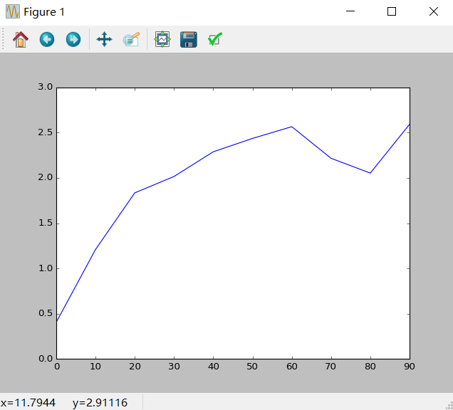
In [78]: df = DataFrame(np.random.randn(10,4).cumsum(0),columns = ['A','B','C','D'],index = np.arange(0,100,10))
In [79]: df.plot()

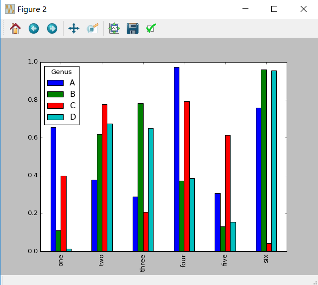
2）柱状图

In [80]:fig,axes = plt.subplots(2,1)
In [81]:data = Series(np.random.rand(16),index=list('abcdefghijklmnop'))

In [82]:data.plot(kind = 'bar',ax = axes[0],color = 'k',alpha = 0.7)
In [83]:data.plot(kind = 'barh',ax = axes[1],color = 'k',alpha = 0.7)

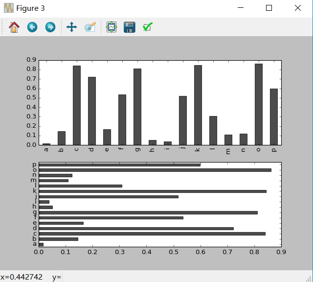
In [84]:df = DataFrame(np.random.rand(6,4),index = ['one','two','three','four','five','six'],columns = pd.Index(['A','B','C','D'],name = 'Genus'))
In [85]:df.plot(kind = 'bar')

3）密度图

In [87]:comp1 = np.random.normal(0,1,size  = 100)
In [88]:comp2 = np.random.normal(10,2,size  = 100)

In [89]:values = Series(np.concatenate([comp1,comp2]))
In [90]:values.hist(bins = 50,alpha = 0.3,color = 'r',normed = True)
In [91]:values.plot(kind = 'kde',style = 'k--')

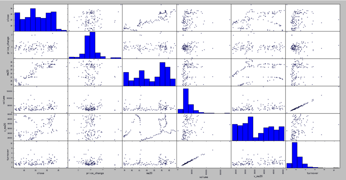
4）散点图

In [7]: import tushare as ts
In [8]: data = ts.get_hist_data('300348',start='2017-08-15')
In [9]: pieces = data[['close', 'price_change', 'ma20','volume', 'v_ma20', 'turnover']]
In [10]: pd.scatter_matrix(pieces)

5）热力图

In [11]: cov = np.corrcoef(pieces.T)
In [12]: img = plt.matshow(cov,cmap=plt.cm.summer)
In [13]: plt.colorbar(img, ticks=[-1,0,1])