机器学习的分类:
有监督学习:
基于连续输出称为回归,如股票预测
基于离散量输出为分类,如数字识别
(常见的有监督学习:回归预测分析,分类;垃圾邮件检测;模式检测;自然语言处理;情绪分析;自动图像分类;自动序列生成等)
无监督的学习:
对象分割,相似性检测,自动标记
强化学习:
(不懂啊,是不是还有一个半监督学习,还是看周志华的机器学习那本吧,现在是意大利的一个人的书)
特征选择与特征工程:
创建训练集和测试集:
训练和测试数据集要满足原始数据分布,并随机混合,避免出现连续元素之间的相关性。
一种将数据分割开为训练和测试的方法如下:0.75:0.25。随机数种子1000,用于再现实验过程等
1 from sklearn.model_selection import train_test_split
2 X_train,X_test,Y_train,Y_test = train_test_split(X,Y,test_size=0.25,random_state=1000)
管理分类数据,将数据转换为数字量等:
#创建
import numpy as np
X = np.random.uniform(0.0,1.0,size=(10,2))
Y = np.random.choice(('Male','Female'),size=(10))
#管理,输出为数字量表示
from sklearn.preprocessing import LabelEncoder
le = LabelEncoder()
yt = le.fit_transform(Y)
print(yt)
获得反向的数据:
output = [1,0,1,1,0,0]
decoded_output = [le.classes_[i] for i in output]
decoded_output
其他方法的编码,如独热编码:每个数据标签转化为一个数组,数组为只有一个特征为1其它为0的数组量:
from sklearn.preprocessing import LabelBinarizer
lb = LabelBinarizer()
Yb = lb.fit_transform(Y)
Yb#独热编码
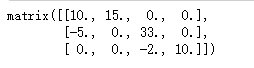
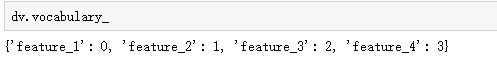
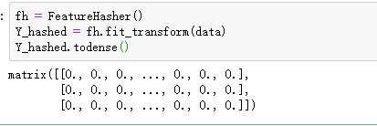
数据量较小时,还可以采用其它编码:
data = [
    {'feature_1':10.0,'feature_2':15.0},
    {'feature_1':-5.0,'feature_3':33.0},
    {'feature_3':-2.0,'feature_4':10.0}
]
from sklearn.feature_extraction import DictVectorizer,FeatureHasher
dv = DictVectorizer()
Y_dict = dv.fit_transform(data)
Y_dict.todense()
#可以产生稀疏矩阵
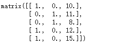
使用oneHotEncoding提供的独热编码:第一个数字进行了编码:
from sklearn.preprocessing import OneHotEncoder
data1 = [
    [0, 10],
    [1, 11],
    [1, 8],
    [0, 12],
    [0, 15]
]
oh = OneHotEncoder(categorical_features=[0])
Y_oh = oh.fit_transform(data1)
Y_oh.todense()
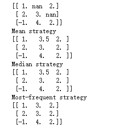
管理缺失特征:对缺失的数据进行平均值,中值,频率的补全
import numpy as np
from sklearn.preprocessing import Imputer
data = np.array([[1, np.nan, 2], [2, 3, np.nan], [-1, 4, 2]])
print(data)
# Imputer with mean-strategy
print('Mean strategy')
imp = Imputer(strategy='mean')
print(imp.fit_transform(data))
# Imputer with median-strategy
print('Median strategy')
imp = Imputer(strategy='median')
print(imp.fit_transform(data))
# Imputer with most-frequent-strategy
print('Most-frequent strategy')
imp = Imputer(strategy='most_frequent')
print(imp.fit_transform(data))
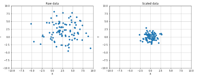
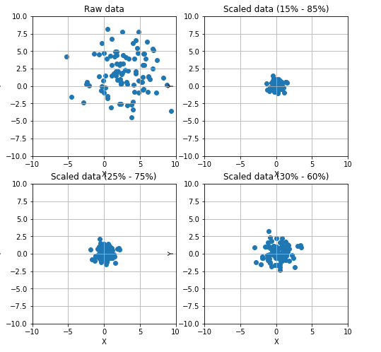
数据缩放和归一化:


 1 from __future__ import print_function
 2 import numpy as np
 3 import matplotlib.pyplot as plt
 4 from sklearn.preprocessing import StandardScaler, RobustScaler
 5 # For reproducibility
 6 np.random.seed(1000)
 7 if __name__ == '__main__':
 8     # Create a dummy dataset
 9     data = np.ndarray(shape=(100, 2))
10     for i in range(100):
11         data[i, 0] = 2.0 + np.random.normal(1.5, 3.0)
12         data[i, 1] = 0.5 + np.random.normal(1.5, 3.0)
13     # Show the original and the scaled dataset
14     fig, ax = plt.subplots(1, 2, figsize=(14, 5))
15
16     ax[0].scatter(data[:, 0], data[:, 1])
17     ax[0].set_xlim([-10, 10])
18     ax[0].set_ylim([-10, 10])
19     ax[0].grid()
20     ax[0].set_xlabel('X')
21     ax[0].set_ylabel('Y')
22     ax[0].set_title('Raw data')
23
24     # Scale data
25     ss = StandardScaler()
26     scaled_data = ss.fit_transform(data)
27
28     ax[1].scatter(scaled_data[:, 0], scaled_data[:, 1])
29     ax[1].set_xlim([-10, 10])
30     ax[1].set_ylim([-10, 10])
31     ax[1].grid()
32     ax[1].set_xlabel('X')
33     ax[1].set_ylabel('Y')
34     ax[1].set_title('Scaled data')
35
36     plt.show()
37
38     # Scale data using a Robust Scaler
39     fig, ax = plt.subplots(2, 2, figsize=(8, 8))
40
41     ax[0, 0].scatter(data[:, 0], data[:, 1])
42     ax[0, 0].set_xlim([-10, 10])
43     ax[0, 0].set_ylim([-10, 10])
44     ax[0, 0].grid()
45     ax[0, 0].set_xlabel('X')
46     ax[0, 0].set_ylabel('Y')
47     ax[0, 0].set_title('Raw data')
48
49     rs = RobustScaler(quantile_range=(15, 85))
50     scaled_data = rs.fit_transform(data)
51
52     ax[0, 1].scatter(scaled_data[:, 0], scaled_data[:, 1])
53     ax[0, 1].set_xlim([-10, 10])
54     ax[0, 1].set_ylim([-10, 10])
55     ax[0, 1].grid()
56     ax[0, 1].set_xlabel('X')
57     ax[0, 1].set_ylabel('Y')
58     ax[0, 1].set_title('Scaled data (15% - 85%)')
59
60     rs1 = RobustScaler(quantile_range=(25, 75))
61     scaled_data1 = rs1.fit_transform(data)
62
63     ax[1, 0].scatter(scaled_data1[:, 0], scaled_data1[:, 1])
64     ax[1, 0].set_xlim([-10, 10])
65     ax[1, 0].set_ylim([-10, 10])
66     ax[1, 0].grid()
67     ax[1, 0].set_xlabel('X')
68     ax[1, 0].set_ylabel('Y')
69     ax[1, 0].set_title('Scaled data (25% - 75%)')
70
71     rs2 = RobustScaler(quantile_range=(30, 65))
72     scaled_data2 = rs2.fit_transform(data)
73
74     ax[1, 1].scatter(scaled_data2[:, 0], scaled_data2[:, 1])
75     ax[1, 1].set_xlim([-10, 10])
76     ax[1, 1].set_ylim([-10, 10])
77     ax[1, 1].grid()
78     ax[1, 1].set_xlabel('X')
79     ax[1, 1].set_ylabel('Y')
80     ax[1, 1].set_title('Scaled data (30% - 60%)')
81
82     plt.show()
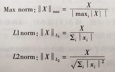
其中的Max L1 L2的缩放定义如下:
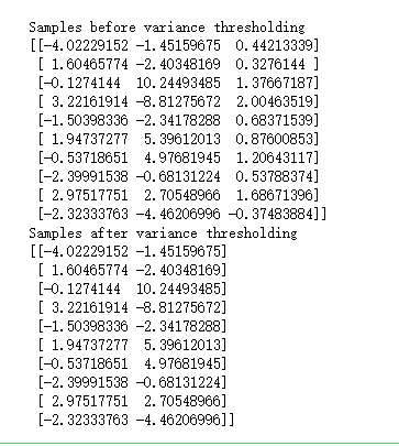
特征选择和过滤:过滤掉信息量比较少的变量:
 1 from __future__ import print_function
 2
 3 import numpy as np
 4 import matplotlib.pyplot as plt
 5
 6 from sklearn.feature_selection import VarianceThreshold
 7
 8 # For reproducibility
 9 np.random.seed(1000)
10
11 if __name__ == '__main__':
12     # Create a dummy dataset
13     X = np.ndarray(shape=(100, 3))
14
15     X[:, 0] = np.random.normal(0.0, 5.0, size=100)
16     X[:, 1] = np.random.normal(0.5, 5.0, size=100)
17     X[:, 2] = np.random.normal(1.0, 0.5, size=100)
18
19     # Show the dataset
20     fig, ax = plt.subplots(1, 1, figsize=(12, 8))
21     ax.grid()
22     ax.set_xlabel('X')
23     ax.set_ylabel('Y')
24
25     ax.plot(X[:, 0], label='STD = 5.0')
26     ax.plot(X[:, 1], label='STD = 5.0')
27     ax.plot(X[:, 2], label='STD = 0.5')
28
29     plt.legend()
30     plt.show()
31
32     # Impose a variance threshold
33     print('Samples before variance thresholding')
34     print(X[0:10, :])
35
36     vt = VarianceThreshold(threshold=1.5)
37     X_t = vt.fit_transform(X)
38
39     # After the filter has removed the componenents
40     print('Samples after variance thresholding')
41     print(X_t[0:10, :])
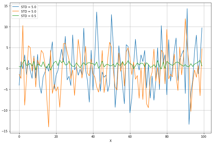
第三列是方差小的那一列,所以第三列被去掉了:
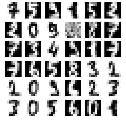
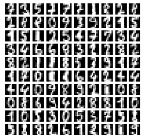
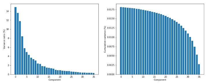
对MNIST做主成分分析!:
 1 from __future__ import print_function
 2
 3 import numpy as np
 4 import matplotlib.pyplot as plt
 5
 6 from sklearn.datasets import load_digits
 7 from sklearn.decomposition import PCA
 8
 9 # For reproducibility
10 np.random.seed(1000)
11
12 if __name__ == '__main__':
13     # Load MNIST digits
14     digits = load_digits()
15
16     # Show some random digits
17     selection = np.random.randint(0, 1797, size=100)
18
19     fig, ax = plt.subplots(10, 10, figsize=(10, 10))
20
21     samples = [digits.data[x].reshape((8, 8)) for x in selection]
22
23     for i in range(10):
24         for j in range(10):
25             ax[i, j].set_axis_off()
26             ax[i, j].imshow(samples[(i * 8) + j], cmap='gray')
27
28     plt.show()
29
30     # Perform a PCA on the digits dataset
31     pca = PCA(n_components=36, whiten=True)
32     X_pca = pca.fit_transform(digits.data / 255)
33
34     print('Explained variance ratio')
35     print(pca.explained_variance_ratio_)
36
37     # Plot the explained variance ratio
38     fig, ax = plt.subplots(1, 2, figsize=(16, 6))
39
40     ax[0].set_xlabel('Component')
41     ax[0].set_ylabel('Variance ratio (%)')
42     ax[0].bar(np.arange(36), pca.explained_variance_ratio_ * 100.0)
43
44     ax[1].set_xlabel('Component')
45     ax[1].set_ylabel('Cumulative variance (%)')
46     ax[1].bar(np.arange(36), np.cumsum(pca.explained_variance_)[::-1])
47
48     plt.show()
49
50     # Rebuild from PCA and show the result
51     fig, ax = plt.subplots(10, 10, figsize=(10, 10))
52
53     samples = [pca.inverse_transform(X_pca[x]).reshape((8, 8)) for x in selection]
54
55     for i in range(10):
56         for j in range(10):
57             ax[i, j].set_axis_off()
58             ax[i, j].imshow(samples[(i * 8) + j], cmap='gray')
59
60     plt.show()
原图:64维,8X8点图,
方差比和累计方差:
pca = PCA(n_components=36, whiten=True)
X_pca = pca.fit_transform(digits.data / 255)
samples = [pca.inverse_transform(X_pca[x]).reshape((8, 8)) for x in selection]
做逆变换投射到原始空间后的图:

非负矩阵分解:当数据集由非负元素组成时:例子如下:
1 from sklearn.datasets import load_iris
2 from sklearn.decomposition import NMF
3 iris = load_iris()
4 iris.data.shape
5
6 iris.data[0:5]
7 Xt[0:5]
8 nmf.inverse_transform(Xt[0:5])

核PCA:可以对非线性的数据集分类,包含比较复杂的数学公式:
 1 from __future__ import print_function
 2
 3 import numpy as np
 4 import matplotlib.pyplot as plt
 5
 6 from sklearn.datasets.samples_generator import make_blobs
 7 from sklearn.decomposition import KernelPCA
 8
 9 # For reproducibility
10 np.random.seed(1000)
11
12 if __name__ == '__main__':
13     # Create a dummy dataset
14     Xb, Yb = make_blobs(n_samples=500, centers=3, n_features=3)
15
16     # Show the dataset
17     fig, ax = plt.subplots(1, 1, figsize=(8, 8))
18     ax.scatter(Xb[:, 0], Xb[:, 1])
19     ax.set_xlabel('X')
20     ax.set_ylabel('Y')
21     ax.grid()
22
23     plt.show()
24
25     # Perform a kernel PCA (with radial basis function)
26     kpca = KernelPCA(n_components=2, kernel='rbf', fit_inverse_transform=True)
27     X_kpca = kpca.fit_transform(Xb)
28
29     # Plot the dataset after PCA
30     fig, ax = plt.subplots(1, 1, figsize=(8, 8))
31     ax.scatter(kpca.X_transformed_fit_[:, 0], kpca.X_transformed_fit_[:, 1])
32     ax.set_xlabel('First component: Variance')
33     ax.set_ylabel('Second component: Mean')
34     ax.grid()
35
36     plt.show()

原子提取和字典学习:类似主成分,从原子的稀疏字典重建样本。
 1 from __future__ import print_function
 2 import numpy as np
 3 import matplotlib.pyplot as plt
 4 from sklearn.datasets import load_digits
 5 from sklearn.decomposition import DictionaryLearning
 6
 7 # For reproducibility
 8 np.random.seed(1000)
 9
10 if __name__ == '__main__':
11     # Load MNIST digits
12     digits = load_digits()
13
14     # Perform a dictionary learning (and atom extraction) from the MNIST dataset
15     dl = DictionaryLearning(n_components=36, fit_algorithm='lars', transform_algorithm='lasso_lars')
16     X_dict = dl.fit_transform(digits.data[0:35])
17
18     # Show the atoms that have been extracted
19     fig, ax = plt.subplots(6, 6, figsize=(8, 8))
20
21     samples = [dl.components_[x].reshape((8, 8)) for x in range(34)]
22
23     for i in range(6):
24         for j in range(6):
25             ax[i, j].set_axis_off()
26             ax[i, j].imshow(samples[(i * 5) + j], cmap='gray')
27
28     plt.show()
结果: