前面已经做了类别和连续特征的分析,本文将针对特征工程进行
导入数据
import pandas as pd
import numpy as np
import matplotlib
import matplotlib.pyplot as plt
import seaborn as sns
%matplotlib inline

#导入训练集和测试集
train_data =pd.read_csv('F:\python\天池_二手车交易价格预测\used_car_train_20200313.csv',sep=' ')
test_data=pd.read_csv('F:\python\天池_二手车交易价格预测\used_car_testB_20200421.csv',sep=' ')
删除异常值
#异常值处理
def out_proc(data,col_name,scale=3):

    def box_plot_out(data_ser,box_scale):
        '''
        data_ser接受pd.Series数据格式
        '''
        iqr=box_scale*(data_ser.quantile(0.75)-data_ser.quantile(0.25))   #0.75分位数的值-0.25分位数的值
        val_low=data_ser.quantile(0.25)-iqr
        val_up=data_ser.quantile(0.75) + iqr
        rule_low = (data_ser < val_low)
        rule_up = (data_ser > val_up)
        return (rule_low, rule_up), (val_low, val_up)  #前面返回异常的pandas.Series 数据,后面返回临界值
    data_n=data.copy()  #先复制一个df
    data_series=data_n[col_name]  #某一列的值
    rule, value = box_plot_out(data_series, box_scale=scale)
    index = np.arange(data_series.shape[0])[rule[0] | rule[1]]  #shape[0]是行数,丨是or的意思,真个就是输出有异常值的索引数
    print("Delete number is: {}".format(len(index)))   #输出异常值个数
    data_n = data_n.drop(index)   #删除异常值
    data_n.reset_index(drop=True, inplace=True)  #重新设置索引
    print("Now column number is: {}".format(data_n.shape[0]))  #删除异常值之后数值的个数
    index_low = np.arange(data_series.shape[0])[rule[0]]   #低于临界值的索引数
    outliers = data_series.iloc[index_low]   #低于临界值的值
    print("Description of data less than the lower bound is:")
    print(pd.Series(outliers).describe())
    index_up = np.arange(data_series.shape[0])[rule[1]]
    outliers = data_series.iloc[index_up]
    print("Description of data larger than the upper bound is:")
    print(pd.Series(outliers).describe())

    fig, ax = plt.subplots(1, 2, figsize=(10, 7))
    sns.boxplot(y=data[col_name], data=data, palette="Set1", ax=ax[0])  #某列原来的箱型图
    sns.boxplot(y=data_n[col_name], data=data_n, palette="Set1", ax=ax[1])  #删除异常值后的箱型图
    return data_n  #返回删除后的值
train_data根据power删除一些异常值
# 这里删不删同学可以自行判断
# 但是要注意 test 的数据不能删 = = 不能掩耳盗铃是不是
train_data= out_proc(train_data,'power',scale=3)

train_data.shape
训练集和测试集放在一起,方便构造特征
#用一列做标签区分一下训练集和测试集
train_data['train']=1
test_data['train']=0
data = pd.concat([train_data, test_data], ignore_index=True)
创建汽车使用时间(data['creatDate'] - data['regDate'])
# 不过要注意,数据里有时间出错的格式,所以我们需要 errors='coerce'
data['used_time'] = (pd.to_datetime(data['creatDate'], format='%Y%m%d', errors='coerce') -
                            pd.to_datetime(data['regDate'], format='%Y%m%d', errors='coerce')).dt.days
由于有些样本有问题,导致使用时间为空,我们计算一下空值的个数
data['used_time'].isnull().sum() #15054
计算某个特征的数据统计量
count_data=train_data.groupby('brand')
all_info={}
for kind,kind_data in count_data:
    info={}
    kind_data=kind_data[kind_data['price']>0] #选出价格大于0的数值
    info['brand_amount']=len(kind_data) #每个分组中价格大于0有多少行数据
    info['brand_price_max']=kind_data.price.max()
    info['brand_price_median'] = kind_data.price.median()
    info['brand_price_min'] = kind_data.price.min()
    info['brand_price_sum'] = kind_data.price.sum()
    info['brand_price_std'] = kind_data.price.std()
    info['brand_price_average'] = round(kind_data.price.sum() / (len(kind_data) + 1), 2)
    all_info[kind] = info   #每个kind的详细数据硬录入里面,这就要分清楚for循环中,变量在里面和在外面的区别
得到的all_info如下:
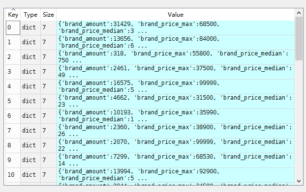
#对于这种value种还有ke的字典,可以使用pd.DataFrame转换成df
brand_fe = pd.DataFrame(all_info).T.reset_index().rename(columns={"index": "brand"})  #转置,重新设索引,只是为了后面和表连接起来
data=data.merge(brand_fe,how='left',on='brand')
数据分箱的好处:
1. 离散后稀疏向量内积乘法运算速度更快,计算结果也方便存储,容易扩展;
2. 离散后的特征对异常值更具鲁棒性,如 age>30 为 1 否则为 0,对于年龄为 200 的也不会对模型造成很大的干扰;
3. LR 属于广义线性模型,表达能力有限,经过离散化后,每个变量有单独的权重,这相当于引入了非线性,能够提升模型的表达能力,加大拟合;
4. 离散后特征可以进行特征交叉,提升表达能力,由 M+N 个变量编程 M*N 个变量,进一步引入非线形,提升了表达能力;
5. 特征离散后模型更稳定,如用户年龄区间,不会因为用户年龄长了一岁就变化
#power分箱
bin=[i*10 for i in range(31)]
data['power_bin']=pd.cut(data['power'],bins=bin,labels=False)  #nan值超出范围了
删除不需要的特征
data = data.drop(['creatDate', 'regDate', 'regionCode'], axis=1)
保存数据,给树模型使用
# 目前的数据其实已经可以给树模型使用了,所以我们导出一下
data.to_csv('data_for_tree.csv', index=0)
构造一份特征给 LR NN 之类的模型用,之所以分开构造是因为,不同模型对数据集的要求不同
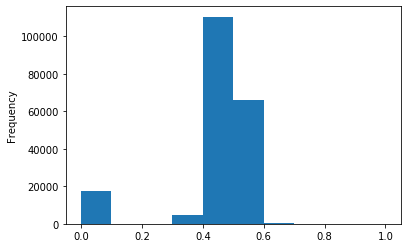
#先取log,在做归一化
data['power']=np.log(data['power']+1)
data['power']=(data['power']-data['power'].min())/(data['power'].max()-data['power'].min())

data['power'].plot.hist()
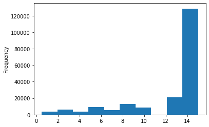
#这个原数据就已经分过箱了,就不需要分箱了
data['kilometer'].plot.hist()
#可以直接归一化
data['kilometer']=(data['kilometer']-data['kilometer'].min())/(data['kilometer'].max()-data['kilometer'].min())
刚才构造的数据统计量也要归一化
# 除此之外 还有我们刚刚构造的统计量特征:
# 'brand_amount', 'brand_price_average', 'brand_price_max',
# 'brand_price_median', 'brand_price_min', 'brand_price_std',
# 'brand_price_sum'
# 这里不再一一举例分析了,直接做变换,
def max_min(x):
    return (x - np.min(x)) / (np.max(x) - np.min(x))

data['brand_amount'] = ((data['brand_amount'] - np.min(data['brand_amount'])) /
                        (np.max(data['brand_amount']) - np.min(data['brand_amount'])))
data['brand_price_average'] = ((data['brand_price_average'] - np.min(data['brand_price_average'])) /
                               (np.max(data['brand_price_average']) - np.min(data['brand_price_average'])))
data['brand_price_max'] = ((data['brand_price_max'] - np.min(data['brand_price_max'])) /
                           (np.max(data['brand_price_max']) - np.min(data['brand_price_max'])))
data['brand_price_median'] = ((data['brand_price_median'] - np.min(data['brand_price_median'])) /
                              (np.max(data['brand_price_median']) - np.min(data['brand_price_median'])))
data['brand_price_min'] = ((data['brand_price_min'] - np.min(data['brand_price_min'])) /
                           (np.max(data['brand_price_min']) - np.min(data['brand_price_min'])))
data['brand_price_std'] = ((data['brand_price_std'] - np.min(data['brand_price_std'])) /
                           (np.max(data['brand_price_std']) - np.min(data['brand_price_std'])))
data['brand_price_sum'] = ((data['brand_price_sum'] - np.min(data['brand_price_sum'])) /
                           (np.max(data['brand_price_sum']) - np.min(data['brand_price_sum'])))
对类别特征要进行独热编码
# 对类别特征进行 OneEncoder
data = pd.get_dummies(data, columns=['model', 'brand', 'bodyType', 'fuelType',
                                     'gearbox', 'notRepairedDamage', 'power_bin'])
保存数据,留给LR使用
# 这份数据可以给 LR 用
data.to_csv('data_for_lr.csv', index=0)
特征构造完毕,特征刷选
相关分析
data.corr()['price'].sort_values()