第三版本
我们前面已经有两个版本了,都涉及到woe转换之类的,现在我们尝试一下xgboost版本的,不需要做woe转换
import numpy as np # linear algebra
import pandas as pd # data processing, CSV file I/O (e.g. pd.read_csv)


from sklearn import preprocessing
from sklearn import metrics
from sklearn import model_selection
from sklearn import ensemble
from sklearn import tree
from sklearn import linear_model
import os, datetime, sys, random, time
import seaborn as sns
import xgboost as xgs
import lightgbm as lgb
import matplotlib.pyplot as plt
import matplotlib.gridspec as gridspec
#from mlxtend import classifier
plt.style.use('fivethirtyeight')
%matplotlib inline
import warnings
warnings.filterwarnings('ignore')
from scipy import stats, special
#import shap
import catboost as ctb

trainingData = pd.read_csv('F:\python\Give-me-some-credit-master\data\cs-training.csv')
testData = pd.read_csv('F:\python\Give-me-some-credit-master\data\cs-test.csv')
探索性分析
trainingData.head()
trainingData.info()
trainingData.describe()
print(trainingData.shape)
print(testData.shape)
testData.head()
testData.info()
testData.describe()
复制原数据
以后要养成在做数据基本分布之后就复制一份数据,避免修改原数据
finalTrain = trainingData.copy()
finalTest = testData.copy()
因为,我们需要预测测试数据中拖欠的概率,所以我们需要首先从中删除附加列
finalTest.drop('SeriousDlqin2yrs', axis=1, inplace = True)
同样如上所述,让我们取ID列,即Unnamed:0,并将其存储在单独的变量中
trainID = finalTrain['Unnamed: 0']
testID = finalTest['Unnamed: 0']

finalTrain.drop('Unnamed: 0', axis=1, inplace=True)
finalTest.drop('Unnamed: 0', axis=1, inplace=True)
y值分布
因为我们有15万的数据。它很有可能是一个不平衡的数据集。因此,检查正负拖欠比率。
fig, axes = plt.subplots(1,2,figsize=(12,6))
finalTrain['SeriousDlqin2yrs'].value_counts().plot.pie(explode=[0,0.1],autopct='%1.1f%%',ax=axes[0])
axes[0].set_title('SeriousDlqin2yrs')
#ax[0].set_ylabel('')
sns.countplot('SeriousDlqin2yrs',data=finalTrain,ax=axes[1])
axes[1].set_title('SeriousDlqin2yrs')
plt.show()
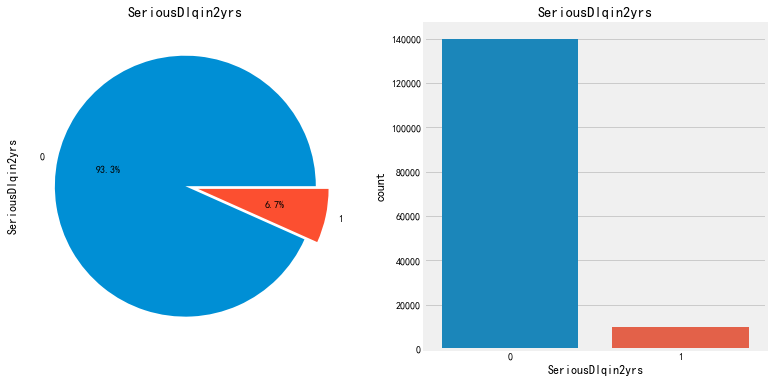
负拖欠与正拖欠异常值的比率为93.3%至6.7%,约为14:1。因此,我们的数据集是高度不平衡的。
我们不能依靠精确分数来预测模型的成功。这里将考虑许多其他的评估指标。但稍后再谈
EDA
现在让我们继续EDA的离群值分析部分。在这里,我们将去除可能影响预测模型的潜在异常值。
异常值分析
fig = plt.figure(figsize=[30,30])
for col,i in zip(finalTrain.columns,range(1,13)):
    axes = fig.add_subplot(7,2,i)
    sns.regplot(finalTrain[col],finalTrain.SeriousDlqin2yrs,ax=axes)
plt.show()
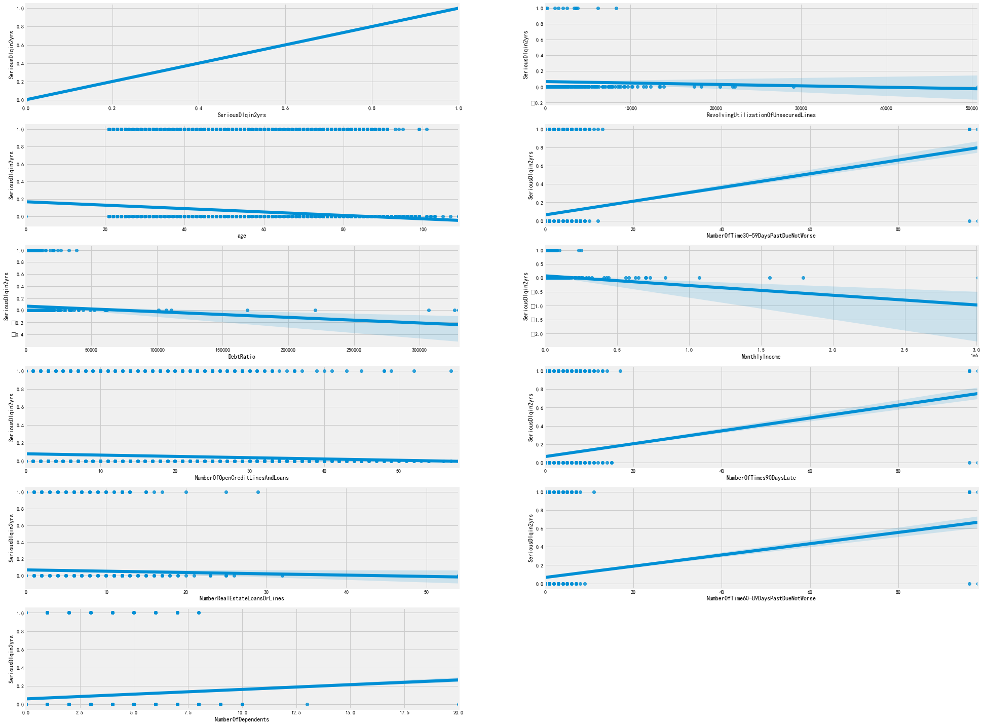
从上图中我们可以观察到:
在NumberOfTime30-59DaysPastDueNotBesters、NumberOfTimes60-89DaysPastDueNotBeare和NumberOfTimes90DaysLate列中,我们可以看到超过90的拖欠范围,这在所有3个功能中都很常见。
有一些不寻常的DebtRatio and RevolvingUtilizationOfUnsecuredLines
第1步:修复NumberOfTime30-59dayspastduenotbears、NumberOfTime60-89dayspastduenotbear和NumberOfTimes90DaysLate列
print("Unique values in '30-59 Days' values that are more than or equal to 90:",np.unique(finalTrain[finalTrain['NumberOfTime30-59DaysPastDueNotWorse']>=90]
                                                                                          ['NumberOfTime30-59DaysPastDueNotWorse']))


print("Unique values in '60-89 Days' when '30-59 Days' values are more than or equal to 90:",np.unique(finalTrain[finalTrain['NumberOfTime30-59DaysPastDueNotWorse']>=90]
                                                                                                       ['NumberOfTime60-89DaysPastDueNotWorse']))


print("Unique values in '90 Days' when '30-59 Days' values are more than or equal to 90:",np.unique(finalTrain[finalTrain['NumberOfTime30-59DaysPastDueNotWorse']>=90]
                                                                                                    ['NumberOfTimes90DaysLate']))


print("Unique values in '60-89 Days' when '30-59 Days' values are less than 90:",np.unique(finalTrain[finalTrain['NumberOfTime30-59DaysPastDueNotWorse']<90]
                                                                                           ['NumberOfTime60-89DaysPastDueNotWorse']))


print("Unique values in '90 Days' when '30-59 Days' values are less than 90:",np.unique(finalTrain[finalTrain['NumberOfTime30-59DaysPastDueNotWorse']<90]
                                                                                        ['NumberOfTimes90DaysLate']))


print("Proportion of positive class with special 96/98 values:",
      round(finalTrain[finalTrain['NumberOfTime30-59DaysPastDueNotWorse']>=90]['SeriousDlqin2yrs'].sum()*100/
      len(finalTrain[finalTrain['NumberOfTime30-59DaysPastDueNotWorse']>=90]['SeriousDlqin2yrs']),2),'%')
Unique values in '30-59 Days' values that are more than or equal to 90: [96 98]
Unique values in '60-89 Days' when '30-59 Days' values are more than or equal to 90: [96 98]
Unique values in '90 Days' when '30-59 Days' values are more than or equal to 90: [96 98]
Unique values in '60-89 Days' when '30-59 Days' values are less than 90: [ 0  1  2  3  4  5  6  7  8  9 11]
Unique values in '90 Days' when '30-59 Days' values are less than 90: [ 0  1  2  3  4  5  6  7  8  9 10 11 12 13 14 15 17]
Proportion of positive class with special 96/98 values: 54.65 %
从下面我们可以看出,当“NumberOfTime30-59DaysPastDueNotBears”列中的记录超过90时,
其他记录逾期付款次数X天的列也具有相同的值。我们将这些分类为特殊标签,因为阳性的比例异常高达54.65%。
这96和98个值可以被视为会计错误。因此,我们将用96之前的最大值替换它们,即13、11和17
loc下面的用法是对应的行列,首先》=90选出对应的行,后面选择的是对应的列
finalTrain.loc[finalTrain['NumberOfTime30-59DaysPastDueNotWorse'] >= 90, 'NumberOfTime30-59DaysPastDueNotWorse'] = 13
finalTrain.loc[finalTrain['NumberOfTime60-89DaysPastDueNotWorse'] >= 90, 'NumberOfTime60-89DaysPastDueNotWorse'] = 11
finalTrain.loc[finalTrain['NumberOfTimes90DaysLate'] >= 90, 'NumberOfTimes90DaysLate'] = 17
print("Unique values in 30-59Days", np.unique(finalTrain['NumberOfTime30-59DaysPastDueNotWorse']))
print("Unique values in 60-89Days", np.unique(finalTrain['NumberOfTime60-89DaysPastDueNotWorse']))
print("Unique values in 90Days", np.unique(finalTrain['NumberOfTimes90DaysLate']))
Unique values in 30-59Days [ 0  1  2  3  4  5  6  7  8  9 10 11 12 13]
Unique values in 60-89Days [ 0  1  2  3  4  5  6  7  8  9 11]
Unique values in 90Days [ 0  1  2  3  4  5  6  7  8  9 10 11 12 13 14 15 17]

测试集处理
print("Unique values in '30-59 Days' values that are more than or equal to 90:",np.unique(finalTest[finalTest['NumberOfTime30-59DaysPastDueNotWorse']>=90]
                                                                                          ['NumberOfTime30-59DaysPastDueNotWorse']))


print("Unique values in '60-89 Days' when '30-59 Days' values are more than or equal to 90:",np.unique(finalTest[finalTest['NumberOfTime30-59DaysPastDueNotWorse']>=90]
                                                                                                       ['NumberOfTime60-89DaysPastDueNotWorse']))


print("Unique values in '90 Days' when '30-59 Days' values are more than or equal to 90:",np.unique(finalTest[finalTest['NumberOfTime30-59DaysPastDueNotWorse']>=90]
                                                                                                    ['NumberOfTimes90DaysLate']))


print("Unique values in '60-89 Days' when '30-59 Days' values are less than 90:",np.unique(finalTest[finalTest['NumberOfTime30-59DaysPastDueNotWorse']<90]
                                                                                           ['NumberOfTime60-89DaysPastDueNotWorse']))


print("Unique values in '90 Days' when '30-59 Days' values are less than 90:",np.unique(finalTest[finalTest['NumberOfTime30-59DaysPastDueNotWorse']<90]
                                                                                        ['NumberOfTimes90DaysLate']))
Unique values in '30-59 Days' values that are more than or equal to 90: [96 98]
Unique values in '60-89 Days' when '30-59 Days' values are more than or equal to 90: [96 98]
Unique values in '90 Days' when '30-59 Days' values are more than or equal to 90: [96 98]
Unique values in '60-89 Days' when '30-59 Days' values are less than 90: [0 1 2 3 4 5 6 7 8 9]
Unique values in '90 Days' when '30-59 Days' values are less than 90: [ 0  1  2  3  4  5  6  7  8  9 10 11 12 16 17 18]
finalTest.loc[finalTest['NumberOfTime30-59DaysPastDueNotWorse'] >= 90, 'NumberOfTime30-59DaysPastDueNotWorse'] = 19
finalTest.loc[finalTest['NumberOfTime60-89DaysPastDueNotWorse'] >= 90, 'NumberOfTime60-89DaysPastDueNotWorse'] = 9
finalTest.loc[finalTest['NumberOfTimes90DaysLate'] >= 90, 'NumberOfTimes90DaysLate'] = 18

print("Unique values in 30-59Days", np.unique(finalTest['NumberOfTime30-59DaysPastDueNotWorse']))
print("Unique values in 60-89Days", np.unique(finalTest['NumberOfTime60-89DaysPastDueNotWorse']))
print("Unique values in 90Days", np.unique(finalTest['NumberOfTimes90DaysLate']))
Unique values in 30-59Days [ 0  1  2  3  4  5  6  7  8  9 10 11 12 19]
Unique values in 60-89Days [0 1 2 3 4 5 6 7 8 9]
Unique values in 90Days [ 0  1  2  3  4  5  6  7  8  9 10 11 12 16 17 18]
第二步:检查 DebtRatio and RevolvingUtilizationOfUnsecuredLines.
print('Debt Ratio:
',finalTrain['DebtRatio'].describe())
print('
Revolving Utilization of Unsecured Lines:
',finalTrain['RevolvingUtilizationOfUnsecuredLines'].describe())
Debt Ratio:
 count    150000.000000
mean        353.005076
std        2037.818523
min           0.000000
25%           0.175074
50%           0.366508
75%           0.868254
max      329664.000000
Name: DebtRatio, dtype: float64

Revolving Utilization of Unsecured Lines:
 count    150000.000000
mean          6.048438
std         249.755371
min           0.000000
25%           0.029867
50%           0.154181
75%           0.559046
max       50708.000000
Name: RevolvingUtilizationOfUnsecuredLines, dtype: float64
在这里你可以看到75分位和最大值之间的巨大差异。让我们更深入地探讨一下
quantiles = [0.75,0.8,0.81,0.85,0.9,0.95,0.975,0.99]

for i in quantiles:
    print(i*100,'% quantile of debt ratio is: ',finalTrain.DebtRatio.quantile(i))
75.0 % quantile of debt ratio is:  0.86825377325
80.0 % quantile of debt ratio is:  4.0
81.0 % quantile of debt ratio is:  14.0
85.0 % quantile of debt ratio is:  269.1499999999942
90.0 % quantile of debt ratio is:  1267.0
95.0 % quantile of debt ratio is:  2449.0
97.5 % quantile of debt ratio is:  3489.024999999994
99.0 % quantile of debt ratio is:  4979.040000000037
正如你所看到的,在81%之后,分位数有了巨大的增长。因此,
我们的主要目标是检查超过81%分位数的潜在异常值。然而,由于我们的数据是150000,
让我们考虑95%和97.5%的分位数进行进一步的分析
finalTrain[finalTrain['DebtRatio'] >= finalTrain['DebtRatio'].quantile(0.95)][['SeriousDlqin2yrs','MonthlyIncome']].describe()
SeriousDlqin2yrs MonthlyIncome
count 7501.000000 379.000000
mean 0.055193 0.084433
std 0.228371 0.278403
min 0.000000 0.000000
25% 0.000000 0.000000
50% 0.000000 0.000000
75% 0.000000 0.000000
max 1.000000 1.000000
我们可以观察到:
在7501名负债率高于95%的客户中,即债务高于收入的次数,只有379人拥有月收入值。
月收入的最大值是1,最小值是0,这让我们怀疑这是数据输入错误。让我们来看看两年严重的拖欠和月收入是否相等
finalTrain[(finalTrain["DebtRatio"] > finalTrain["DebtRatio"].quantile(0.95)) & (finalTrain['SeriousDlqin2yrs'] == finalTrain['MonthlyIncome'])]
因此,我们的疑点是真实的,379排中有331排的月收入等于2年内严重的拖欠。因此,
我们将从我们的分析中删除这些331个异常值,因为它们的当前值对我们的预测建模没有用处,而且会增加偏差和方差。
这背后的原因是,我们有331行的债务比率与客户的收入相比是巨大的,他们没有仔细审查违约,这只是一个数据输入错误
finalTrain = finalTrain[-((finalTrain["DebtRatio"] > finalTrain["DebtRatio"].quantile(0.95)) & (finalTrain['SeriousDlqin2yrs'] == finalTrain['MonthlyIncome']))]
finalTrain
循环使用无担保额度
此字段基本上表示客户信用额度所欠金额的比率。比率高于1将被视为严重违约。
10的比率在功能上似乎也是可能的,让我们看看有多少客户的无担保额度的循环利用率大于10
finalTrain[finalTrain['RevolvingUtilizationOfUnsecuredLines']>10].describe()
在这里,如果你看到第50分位数和75分位数之间的差异,你会发现从13分位数到1891.25分位数有了巨大的增长。
既然13看起来是一个合理的比率(但太高了),让我们检查一下有多少计数在13以上。
finalTrain[finalTrain['RevolvingUtilizationOfUnsecuredLines']>13].describe()
尽管欠了几千,这238人没有显示任何违约,这意味着这可能是另一个错误。即使不是错误,
这些数字也会给我们的最终预测增加巨大的偏差和偏差。因此,最好的决定是删除这些值
finalTrain = finalTrain[finalTrain['RevolvingUtilizationOfUnsecuredLines']<=13]
finalTrain
现在处理异常值。接下来,我们将继续处理丢失的数据,
正如我们在本笔记本的开头所观察到的那样,MonthlyIncome和NumberOfDependents的值为空。
空处理
由于MonthlyIncome是一个整数值,我们将用中值替换null。
如果客户的依赖项的数量不存在,那么就意味着他们的依赖项的数量是可变的。因此,我们用零来填充它们
def MissingHandler(df):
    DataMissing = df.isnull().sum()*100/len(df)
    DataMissingByColumn = pd.DataFrame({'Percentage Nulls':DataMissing})
    DataMissingByColumn.sort_values(by='Percentage Nulls',ascending=False,inplace=True)
    return DataMissingByColumn[DataMissingByColumn['Percentage Nulls']>0]

MissingHandler(finalTrain)
Percentage Nulls
MonthlyIncome 19.850633
NumberOfDependents 2.617261
因此,月收入和家属人数分别为19.76%和2.59%。
finalTrain['MonthlyIncome'].fillna(finalTrain['MonthlyIncome'].median(), inplace=True)
finalTrain['NumberOfDependents'].fillna(0, inplace = True)
重新检查空值
MissingHandler(finalTrain)
测试集
MissingHandler(finalTest)
finalTest['MonthlyIncome'].fillna(finalTrain['MonthlyIncome'].median(), inplace=True)
finalTest['NumberOfDependents'].fillna(0, inplace = True)
MissingHandler(finalTest)
最后行数
print(finalTrain.shape)
print(finalTest.shape)
'''
(149431, 11)
(101503, 10)
'''
附加EDA
让我们研究更多关于数据集的事情,以便更熟悉它。
相关矩阵
fig = plt.figure(figsize = [15,10])
mask = np.zeros_like(finalTrain.corr(), dtype=np.bool)
mask[np.triu_indices_from(mask)] = True
sns.heatmap(finalTrain.corr(), cmap=sns.diverging_palette(150, 275, s=80, l=55, n=9), mask = mask, annot=True, center = 0)
plt.title("Correlation Matrix (HeatMap)", fontsize = 15)

从上面的相关热图中,我们可以看到最相关的值是NumberOfTime30-59dayspastduenotbears,NumberOfTime60-89dayspastduenotbearse和NumberOfTimes90DaysLate。
现在让我们转到笔记本的功能工程部分
特征工程
让我们首先将训练集和测试集结合起来,为数据添加特性并进行进一步的分析。稍后我们将在模型测试之前拆分它们
SeriousDlqIn2Yrs = finalTrain['SeriousDlqin2yrs']

finalTrain.drop('SeriousDlqin2yrs', axis = 1 , inplace = True)
finalData = pd.concat([finalTrain, finalTest])

finalData.shape
#(250934, 10)
添加一些新功能:
月收入:月收入除以受抚养人的数量
月收入乘以负债率
isRetired:月收入为0且年龄大于65岁(假定退休年龄)的人
回笼额度:未结贷款额度与房地产贷款额度之差
hasRevolvingLines:如果RevolvingLines存在,则1其他0
HasMultipleResaleStates:如果不动产数量大于2
收入:月收入除以1000。对于这些人来说,欺诈的可能性更大,也可能意味着这个人有了一份新工作,而且还没有加薪百分之十。这两组人都表示风险更高。
finalData['MonthlyIncomePerPerson'] = finalData['MonthlyIncome']/(finalData['NumberOfDependents']+1)
finalData['MonthlyIncomePerPerson'].fillna(0, inplace=True)

finalData['MonthlyDebt'] = finalData['MonthlyIncome']*finalData['DebtRatio']
finalData['MonthlyDebt'].fillna(finalData['DebtRatio'],inplace=True)
finalData['MonthlyDebt'] = np.where(finalData['MonthlyDebt']==0, finalData['DebtRatio'],finalData['MonthlyDebt'])

finalData['isRetired'] = np.where((finalData['age'] > 65), 1, 0)

finalData['RevolvingLines'] = finalData['NumberOfOpenCreditLinesAndLoans']-finalData['NumberRealEstateLoansOrLines']

finalData['hasRevolvingLines']=np.where((finalData['RevolvingLines']>0),1,0)

finalData['hasMultipleRealEstates'] = np.where((finalData['NumberRealEstateLoansOrLines']>=2),1,0)

finalData['incomeDivByThousand'] = finalData['MonthlyIncome']/1000
finalData.shape
#(250934, 17)
MissingHandler(finalData)
#Percentage Nulls
我们现在已经在数据集中添加了新的特性。接下来,我们将通过分析各个列的分布对数据进行偏斜检查,并执行Box-Cox变换来减少偏斜。
偏度检验与Box-Cox变换
让我们先检查每个值的分布
columnList = list(finalData.columns)
columnList

fig = plt.figure(figsize=[20,20])
for col,i in zip(columnList,range(1,19)):
    axes = fig.add_subplot(6,3,i)
    sns.distplot(finalData[col],ax=axes, kde_kws={'bw':1.5}, color='purple')
plt.show()
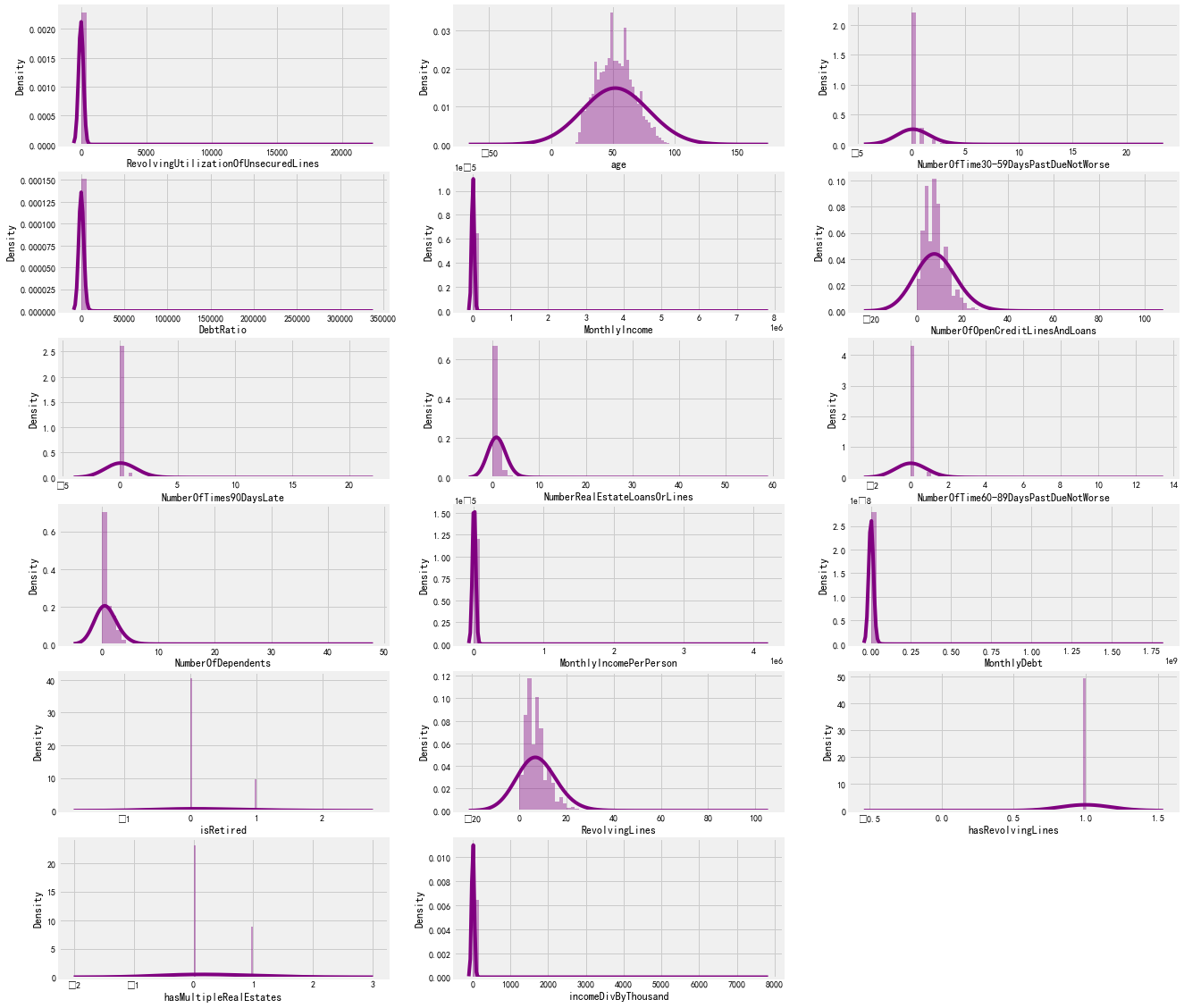
从上面的分布图中,我们可以看到,我们的大部分数据是在任何一个方向上倾斜的。我们只能看到年龄形成接近正态分布。让我们检查每列的倾斜度值
def SkewMeasure(df):
    nonObjectColList = df.dtypes[df.dtypes != 'object'].index
    skewM = df[nonObjectColList].apply(lambda x: stats.skew(x.dropna())).sort_values(ascending = False)
    skewM=pd.DataFrame({'skew':skewM})
    return skewM[abs(skewM)>0.5].dropna()

skewM = SkewMeasure(finalData)
skewM
skew
MonthlyIncome 218.270205
incomeDivByThousand 218.270205
MonthlyIncomePerPerson 206.221804
MonthlyDebt 98.604981
DebtRatio 92.819627
RevolvingUtilizationOfUnsecuredLines 91.721780
NumberOfTimes90DaysLate 15.097509
NumberOfTime60-89DaysPastDueNotWorse 13.509677
NumberOfTime30-59DaysPastDueNotWorse 9.773995
NumberRealEstateLoansOrLines 3.217055
NumberOfDependents 1.829982
isRetired 1.564456
RevolvingLines 1.364633
NumberOfOpenCreditLinesAndLoans 1.219429
hasMultipleRealEstates 1.008475
hasRevolvingLines -8.106007
所有列的倾斜度都非常高。我们将使用λ=0.15的Box-Cox变换来减少这种偏斜
for i in skewM.index:
    finalData[i] = special.boxcox1p(finalData[i],0.15) #lambda = 0.15

SkewMeasure(finalData)
skew
RevolvingUtilizationOfUnsecuredLines 23.234640
NumberOfTimes90DaysLate 6.787000
NumberOfTime60-89DaysPastDueNotWorse 6.602180
NumberOfTime30-59DaysPastDueNotWorse 3.212010
DebtRatio 1.958314
MonthlyDebt 1.817649
isRetired 1.564456
hasMultipleRealEstates 1.008475
NumberOfDependents 0.947591
incomeDivByThousand 0.708168
MonthlyIncomePerPerson -1.558107
MonthlyIncome -2.152376
hasRevolvingLines -8.106007
由于应用了Box-Cox变换,偏度在更高的范围内减小了。让我们再次检查各个列的分布图:
fig = plt.figure(figsize=[20,20])
for col,i in zip(columnList,range(1,19)):
    axes = fig.add_subplot(6,3,i)
    sns.distplot(finalData[col],ax=axes, kde_kws={'bw':1.5}, color='purple')
plt.show()
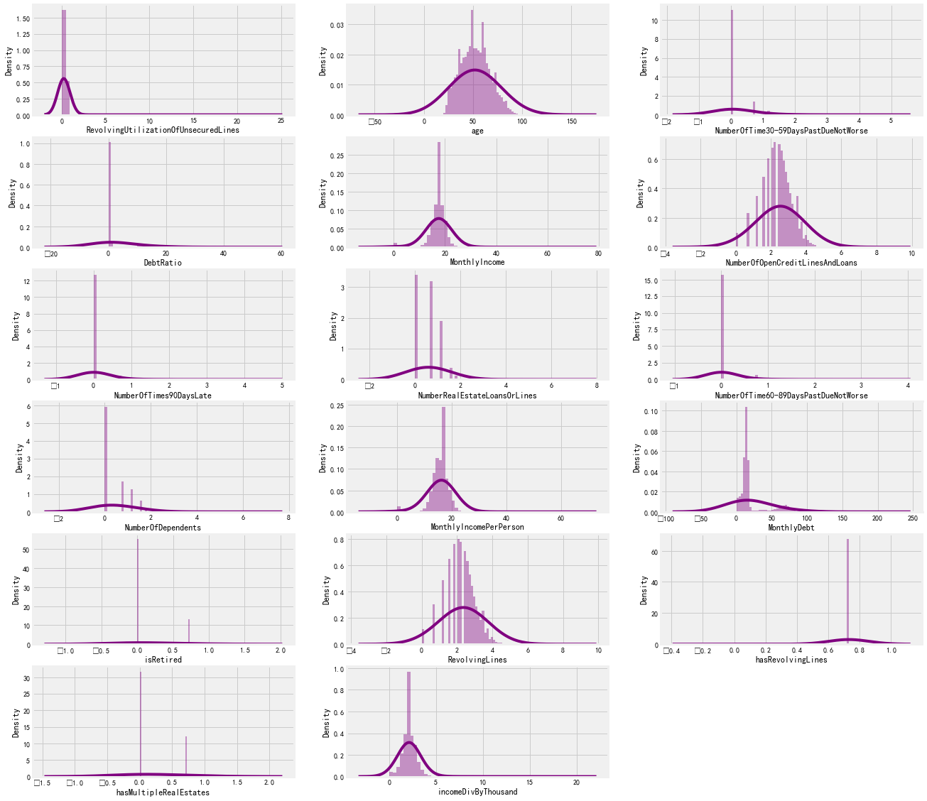
As you can see, our graphs look much better now.
Model Training
Train-Validation Split
We will currently split the train and validation sets into a 70-30 proportion.
trainDF = finalData[:len(finalTrain)]
testDF = finalData[len(finalTrain):]
print(trainDF.shape)
print(testDF.shape)
'''
(149431, 17)
(101503, 17)
'''
xTrain, xTest, yTrain, yTest = model_selection.train_test_split(trainDF.to_numpy(),SeriousDlqIn2Yrs.to_numpy(),test_size=0.3,random_state=2020)
LightGBM
超参数调参
lgbAttributes = lgb.LGBMClassifier(objective='binary', n_jobs=-1, random_state=2020, importance_type='gain')

lgbParameters = {
    'max_depth' : [2,3,4,5],
    'learning_rate': [0.05, 0.1,0.125,0.15],
    'colsample_bytree' : [0.2,0.4,0.6,0.8,1],
    'n_estimators' : [400,500,600,700,800,900],
    'min_split_gain' : [0.15,0.20,0.25,0.3,0.35], #equivalent to gamma in XGBoost
    'subsample': [0.6,0.7,0.8,0.9,1],
    'min_child_weight': [6,7,8,9,10],
    'scale_pos_weight': [10,15,20],
    'min_data_in_leaf' : [100,200,300,400,500,600,700,800,900],
    'num_leaves' : [20,30,40,50,60,70,80,90,100]
}

lgbModel = model_selection.RandomizedSearchCV(lgbAttributes, param_distributions = lgbParameters, cv = 5, random_state=2020)

lgbModel.fit(xTrain,yTrain.flatten(),feature_name=trainDF.columns.to_list())
RandomizedSearchCV(cv=5,
                   estimator=LGBMClassifier(importance_type='gain',
                                            objective='binary',
                                            random_state=2020),
                   param_distributions={'colsample_bytree': [0.2, 0.4, 0.6, 0.8,
                                                             1],
                                        'learning_rate': [0.05, 0.1, 0.125,
                                                          0.15],
                                        'max_depth': [2, 3, 4, 5],
                                        'min_child_weight': [6, 7, 8, 9, 10],
                                        'min_data_in_leaf': [100, 200, 300, 400,
                                                             500, 600, 700, 800,
                                                             900],
                                        'min_split_gain': [0.15, 0.2, 0.25, 0.3,
                                                           0.35],
                                        'n_estimators': [400, 500, 600, 700,
                                                         800, 900],
                                        'num_leaves': [20, 30, 40, 50, 60, 70,
                                                       80, 90, 100],
                                        'scale_pos_weight': [10, 15, 20],
                                        'subsample': [0.6, 0.7, 0.8, 0.9, 1]},
                   random_state=2020)
bestEstimatorLGB = lgbModel.best_estimator_
bestEstimatorLGB
LGBMClassifier(colsample_bytree=0.4, importance_type='gain', max_depth=5,
               min_child_weight=6, min_data_in_leaf=600, min_split_gain=0.25,
               n_estimators=900, num_leaves=50, objective='binary',
               random_state=2020, scale_pos_weight=10, subsample=0.9)
从RandomSearchCV中保存最佳估计量
bestEstimatorLGB = lgb.LGBMClassifier(colsample_bytree=0.4, importance_type='gain', max_depth=5,
               min_child_weight=6, min_data_in_leaf=600, min_split_gain=0.25,
               n_estimators=900, num_leaves=50, objective='binary',
               random_state=2020, scale_pos_weight=10, subsample=0.9).fit(xTrain,yTrain.flatten(),feature_name=trainDF.columns.to_list())
yPredLGB = bestEstimatorLGB.predict_proba(xTest)
yPredLGB = yPredLGB[:,1]
yTestPredLGB = bestEstimatorLGB.predict(xTest)
print(metrics.classification_report(yTest,yTestPredLGB))
              precision    recall  f1-score   support

           0       0.97      0.86      0.92     41956
           1       0.26      0.68      0.37      2973

    accuracy                           0.85     44929
   macro avg       0.62      0.77      0.64     44929
weighted avg       0.93      0.85      0.88     44929
metrics.confusion_matrix(yTest,yTestPredLGB)
array([[36214,  5742],
       [  965,  2008]], dtype=int64)
LGBMMetrics = pd.DataFrame({'Model': 'LightGBM',
                            'MSE': round(metrics.mean_squared_error(yTest, yTestPredLGB)*100,2),
                            'RMSE' : round(np.sqrt(metrics.mean_squared_error(yTest, yTestPredLGB)*100),2),
                            'MAE' : round(metrics.mean_absolute_error(yTest, yTestPredLGB)*100,2),
                            'MSLE' : round(metrics.mean_squared_log_error(yTest, yTestPredLGB)*100,2),
                            'RMSLE' : round(np.sqrt(metrics.mean_squared_log_error(yTest, yTestPredLGB)*100),2),
                            'Accuracy Train' : round(bestEstimatorLGB.score(xTrain, yTrain) * 100,2),
                            'Accuracy Test' : round(bestEstimatorLGB.score(xTest, yTest) * 100,2),
                            'F-Beta Score (β=2)' : round(metrics.fbeta_score(yTest, yTestPredLGB, beta=2)*100,2)},index=[1])

LGBMMetrics
Model MSE RMSE MAE MSLE RMSLE Accuracy Train Accuracy Test F-Beta Score (β=2)
1 LightGBM 14.49 3.81 14.49 6.96 2.64 86.55 85.51 51.35
ROC AUC
fpr,tpr,_ = metrics.roc_curve(yTest,yPredLGB)
rocAuc = metrics.auc(fpr, tpr)
plt.figure(figsize=(12,6))
plt.title('ROC Curve')
sns.lineplot(fpr, tpr, label = 'AUC for LightGBM Model = %0.2f' % rocAuc)
plt.legend(loc = 'lower right')
plt.plot([0, 1], [0, 1],'r--')
plt.ylabel('True Positive Rate')
plt.xlabel('False Positive Rate')
plt.show()

特征重要性
lgb.plot_importance(bestEstimatorLGB, importance_type='gain')

使用SHAP的特征重要性
import shap
X = pd.DataFrame(xTrain, columns=trainDF.columns.to_list())

explainer = shap.TreeExplainer(bestEstimatorLGB)
shap_values = explainer.shap_values(X)

shap.summary_plot(shap_values[1], X)
XGBoost
调参,由于我没有安装CPU版本的,具体请参考https://xgboost.readthedocs.io/en/latest/gpu/index.html,CPU版本的速度会快很多
xgbAttribute = #xgs.XGBClassifier(tree_method='gpu_hist',n_jobs=-1,
gpu_id=0)
#由于我没有安装CPU版本的,所以只能使用非CPU版本的,因此改一下参数
xgs.XGBClassifier(tree_method='hist',n_jobs=-1,
)


xgbParameters = {
    'max_depth' : [2,3,4,5,6,7,8],
    'learning_rate':[0.05,0.1,0.125,0.15],
    'colsample_bytree' : [0.2,0.4,0.6,0.8,1],
    'n_estimators' : [400,500,600,700,800,900],
    'gamma':[0.15,0.20,0.25,0.3,0.35],
    'subsample': [0.6,0.7,0.8,0.9,1],
    'min_child_weight': [6,7,8,9,10],
    'scale_pos_weight': [10,15,20]

}

xgbModel = model_selection.RandomizedSearchCV(xgbAttribute, param_distributions = xgbParameters, cv = 5, random_state=2020)

xgbModel.fit(xTrain,yTrain.flatten())
RandomizedSearchCV(cv=5, estimator=XGBClassifier(n_jobs=-1, tree_method='hist'),
                   param_distributions={'colsample_bytree': [0.2, 0.4, 0.6, 0.8,
                                                             1],
                                        'gamma': [0.15, 0.2, 0.25, 0.3, 0.35],
                                        'learning_rate': [0.05, 0.1, 0.125,
                                                          0.15],
                                        'max_depth': [2, 3, 4, 5, 6, 7, 8],
                                        'min_child_weight': [6, 7, 8, 9, 10],
                                        'n_estimators': [400, 500, 600, 700,
                                                         800, 900],
                                        'scale_pos_weight': [10, 15, 20],
                                        'subsample': [0.6, 0.7, 0.8, 0.9, 1]},
                   random_state=2020)
bestEstimatorXGB = xgbModel.best_estimator_
bestEstimatorXGB
最好的参数是:
XGBClassifier(colsample_bytree=0.4, gamma=0.25, learning_rate=0.125,
              max_depth=5, min_child_weight=9, n_estimators=800, n_jobs=-1,
              scale_pos_weight=10, tree_method='hist')
bestEstimatorXGB = xgs.XGBClassifier(base_score=0.5, booster='gbtree', colsample_bylevel=1,
              colsample_bynode=1, colsample_bytree=0.4, gamma=0.25,
              importance_type='gain', interaction_constraints='',
              learning_rate=0.125, max_delta_step=0, max_depth=5,
              min_child_weight=9,
              monotone_constraints='(0,0,0,0,0,0,0,0,0,0,0,0,0,0,0,0,0,0)',
              n_estimators=800, n_jobs=-1, num_parallel_tree=1, random_state=0,
              reg_alpha=0, reg_lambda=1, scale_pos_weight=10, subsample=1,
              tree_method='hist', validate_parameters=1).fit(xTrain,yTrain.flatten())
yPredXGB = bestEstimatorXGB.predict_proba(xTest)
yPredXGB = yPredXGB[:,1]

yTestPredXGB = bestEstimatorXGB.predict(xTest)
print(metrics.classification_report(yTest,yTestPredXGB))
              precision    recall  f1-score   support

           0       0.97      0.89      0.93     41956
           1       0.28      0.62      0.38      2973

    accuracy                           0.87     44929
   macro avg       0.62      0.75      0.66     44929
weighted avg       0.92      0.87      0.89     44929
混淆矩阵
metrics.confusion_matrix(yTest,yTestPredXGB)
array([[37174,  4782],
       [ 1132,  1841]], dtype=int64)
XGBMetrics = pd.DataFrame({'Model': 'XGBoost',
                            'MSE': round(metrics.mean_squared_error(yTest, yTestPredXGB)*100,2),
                            'RMSE' : round(np.sqrt(metrics.mean_squared_error(yTest, yTestPredXGB)*100),2),
                            'MAE' : round(metrics.mean_absolute_error(yTest, yTestPredXGB)*100,2),
                            'MSLE' : round(metrics.mean_squared_log_error(yTest, yTestPredXGB)*100,2),
                            'RMSLE' : round(np.sqrt(metrics.mean_squared_log_error(yTest, yTestPredXGB)*100),2),
                            'Accuracy Train' : round(bestEstimatorLGB.score(xTrain, yTrain) * 100,2),
                            'Accuracy Test' : round(bestEstimatorLGB.score(xTest, yTest) * 100,2),
                            'F-Beta Score (β=2)' : round(metrics.fbeta_score(yTest, yTestPredXGB, beta=2)*100,2)},index=[2])

XGBMetrics

ROC AUC
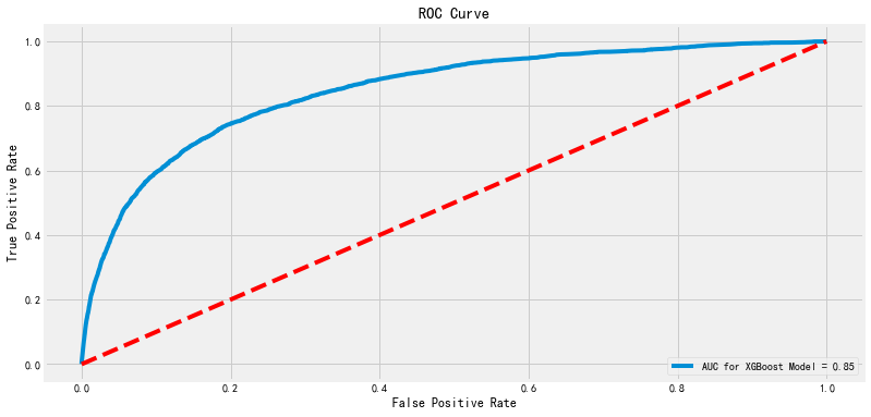
fpr,tpr,_ = metrics.roc_curve(yTest,yPredXGB)
rocAuc = metrics.auc(fpr, tpr)
plt.figure(figsize=(12,6))
plt.title('ROC Curve')
sns.lineplot(fpr, tpr, label = 'AUC for XGBoost Model = %0.2f' % rocAuc)
plt.legend(loc = 'lower right')
plt.plot([0, 1], [0, 1],'r--')
plt.ylabel('True Positive Rate')
plt.xlabel('False Positive Rate')
plt.show()
FEATURE IMPORTANCE
bestEstimatorXGB.get_booster().feature_names = trainDF.columns.to_list()
xgs.plot_importance(bestEstimatorXGB, importance_type='gain')

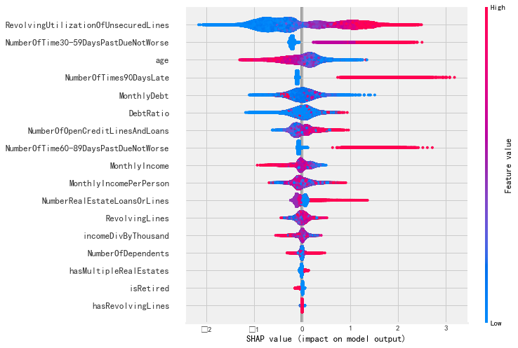
FEATURE IMPORTANCE USING SHAP
mybooster = bestEstimatorXGB.get_booster()
model_bytearray = mybooster.save_raw()[4:]
def myfun(self=None):
    return model_bytearray

mybooster.save_raw = myfun


X = pd.DataFrame(xTrain, columns=trainDF.columns.to_list())

explainer = shap.TreeExplainer(mybooster)
shap_values = explainer.shap_values(X)

shap.summary_plot(shap_values, X)
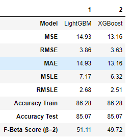
二者比较
frames = [LGBMMetrics, XGBMetrics]
TrainingResult = pd.concat(frames)
TrainingResult.T
LGBM Submission
因为,我们可以看到我们的LGBM表现更好,我们会提交这个。(迟交)
lgbProbs = bestEstimatorLGB.predict_proba(testDF)
lgbDF = pd.DataFrame({'ID': testID, 'Probability': lgbProbs[:,1]})
lgbDF.to_csv('submission.csv', index=False)
#因此拖欠的可能性

lgbDF