信用卡评分模型（四）

数据来源：https://www.kaggle.com/c/GiveMeSomeCredit

 https://www.statsmodels.org/stable/generated/statsmodels.discrete.discrete_model.Logit.html#statsmodels.discrete.discrete_model.Logit

使用statsmodels.api.Logit建模

前面参考了这么多篇文章，现在按照自己平时的思路简单的写了一篇

总结：

1.关于缺失值的问题，首先不用处理，先做iv，再具体要看空值的部分的逾期表现如何，

（1）单独作为一箱：如果逾期率和其他分箱都不接近，或者是异常小，或者异常大，我们就可以单独作为一箱，

（2）均值填充：如果和均值所在的那一箱逾期率接近，则可以用均值填充

（3）中位数填充：如果和中位数所在的那一箱逾期率接近，则可以用中位数填充

（4）使用随机森林模型填充：只要不是上面第一种情况，都可以使用随机森林模型填充

（5）看看是否可以有其他列来补充

2.关于异常值的处理

（1）数值型的类别个数不是很多的话，不建议使用分位数去处理异常值

（2）我们也可以先做iv值，然后在看看箱和箱直接的值得差异，如何差异特别大，即可说明这里面有差异值

（3）差异值是该删除还是修改呢，这得需要我们去判断

3.我们使用woe转化之后还需要做标准化吗？

 

一、statsmodels

具体看代码吧

# -*- coding: utf-8 -*-
"""
Created on Wed Jan 20 19:33:13 2021

@author: Administrator
"""

#%%导入模块
import pandas as pd 
import numpy as np
from scipy import stats
import seaborn as sns
import matplotlib.pyplot as plt
%matplotlib inline
plt.rc("font",family="SimHei",size="12")  #解决中文无法显示的问题

#%%导入数据
train=pd.read_csv('D:python_homeGive-me-some-credit-masterdata\cs-training.csv')

train.shape  #(150000, 12)
train.pop('Unnamed: 0')
train.columns
'''
[ 'SeriousDlqin2yrs',
       'RevolvingUtilizationOfUnsecuredLines', 'age',
       'NumberOfTime30-59DaysPastDueNotWorse', 'DebtRatio', 'MonthlyIncome',
       'NumberOfOpenCreditLinesAndLoans', 'NumberOfTimes90DaysLate',
       'NumberRealEstateLoansOrLines', 'NumberOfTime60-89DaysPastDueNotWorse',
       'NumberOfDependents']

        {'Unnamed: 0':'id',
        'SeriousDlqin2yrs':'好坏客户',
        'RevolvingUtilizationOfUnsecuredLines':'可用额度比值',
        'age':'年龄',
        'NumberOfTime30-59DaysPastDueNotWorse':'逾期30-59天笔数',
        'DebtRatio':'负债率',
        'MonthlyIncome':'月收入',
        'NumberOfOpenCreditLinesAndLoans':'信贷数量',
        'NumberOfTimes90DaysLate':'逾期90天笔数',
        'NumberRealEstateLoansOrLines':'固定资产贷款量',
        'NumberOfTime60-89DaysPastDueNotWorse':'逾期60-89天笔数',
        'NumberOfDependents':'家属数量'}
'''


#%%查看每个变量的唯一值
for i in list(train.columns):
    print(i,'的唯一值是：',train[i].nunique())
    
'''
SeriousDlqin2yrs 的唯一值是： 2
RevolvingUtilizationOfUnsecuredLines 的唯一值是： 125728
age 的唯一值是： 86
NumberOfTime30-59DaysPastDueNotWorse 的唯一值是： 16
DebtRatio 的唯一值是： 114194
MonthlyIncome 的唯一值是： 13594
NumberOfOpenCreditLinesAndLoans 的唯一值是： 58
NumberOfTimes90DaysLate 的唯一值是： 19
NumberRealEstateLoansOrLines 的唯一值是： 28
NumberOfTime60-89DaysPastDueNotWorse 的唯一值是： 13
NumberOfDependents 的唯一值是： 13
'''
#%%查看缺失值
train.isnull().sum()
'''
SeriousDlqin2yrs                            0
RevolvingUtilizationOfUnsecuredLines        0
age                                         0
NumberOfTime30-59DaysPastDueNotWorse        0
DebtRatio                                   0
MonthlyIncome                           29731
NumberOfOpenCreditLinesAndLoans             0
NumberOfTimes90DaysLate                     0
NumberRealEstateLoansOrLines                0
NumberOfTime60-89DaysPastDueNotWorse        0
NumberOfDependents                       3924
dtype: int64
'''
#月收入缺失比例还是很高的，展示不管
#%%按照字面理解。好像都是数值型变量
import pycard as pc
num_iv_woedf = pc.WoeDf()
clf = pc.NumBin()
for i in list(train.columns):
    clf.fit(train[i] ,train.SeriousDlqin2yrs)
    clf.generate_transform_fun()
    num_iv_woedf.append(clf.woe_df_)
num_iv_woedf.to_excel('tmp18')


#上面可知有2个字段是有缺失值得，我们可以将NumberOfDependents填补为-1，收入的填补为均值
train_copy = train.copy()
train_copy.NumberOfDependents[train_copy.NumberOfDependents.isnull()] = -1
train_copy.MonthlyIncome.median()
train_copy.MonthlyIncome[train_copy.MonthlyIncome.isnull()] = 5400.0


#有iv的计算可知 (35.892, inf]    RevolvingUtilizationOfUnsecuredLines，有点问题，删除
train_copy = train_copy[train_copy.RevolvingUtilizationOfUnsecuredLines<=35.892]
train_copy.shape


#%%异常值处理
#我错了，下面这个异常值处理并不合理，不处理了，

#%%分箱
import pycard as pc
num_iv_woedf = pc.WoeDf()
clf = pc.NumBin()
for i in list(train_copy.columns)[1:]:
    clf.fit(train_copy[i] ,train_copy.SeriousDlqin2yrs)
    clf.generate_transform_fun()
    num_iv_woedf.append(clf.woe_df_)





from numpy import *
train_copy['RevolvingUtilizationOfUnsecuredLines_bin'] = pd.cut(train_copy.RevolvingUtilizationOfUnsecuredLines,bins=[-inf, 0.1318, 0.3009, 0.495, 0.6981, 0.8628, 1.0051, 1.0284, inf])
train_copy['age_bin'] = pd.cut(train_copy.age,bins=[-inf, 28.5, 36.5, 43.5, 55.5, 57.5, 62.5, 67.5, inf])
train_copy['NumberOfTime30-59DaysPastDueNotWorse_bin'] = pd.cut(train_copy['NumberOfTime30-59DaysPastDueNotWorse'],bins=[-inf, 0.5, 1.5, 3.5, inf])
train_copy['DebtRatio_bin'] = pd.cut(train_copy.DebtRatio,bins=[-inf, 0.0, 0.0163, 0.4233, 0.6537, 3.9728, 995.5, inf])
train_copy['MonthlyIncome_bin'] = pd.cut(train_copy.MonthlyIncome,bins=[-inf, 270.0, 930.5, 3332.5, 5320.5, 5400.5, 7656.5, 9945.5, inf])
train_copy['NumberOfOpenCreditLinesAndLoans_bin'] = pd.cut(train_copy.NumberOfOpenCreditLinesAndLoans,bins=[-inf, 0.5, 1.5, 2.5, 3.5, 13.5, inf])
train_copy['NumberOfTimes90DaysLate_bin'] = pd.cut(train_copy.NumberOfTimes90DaysLate,bins=[-inf, 0.5, 1.5, 2.5, inf])
train_copy['NumberRealEstateLoansOrLines_bin'] = pd.cut(train_copy.NumberRealEstateLoansOrLines,bins=[-inf, 0.5, 2.5, 4.5, 6.5, inf])
train_copy['NumberOfTime60-89DaysPastDueNotWorse_bin'] = pd.cut(train_copy['NumberOfTime60-89DaysPastDueNotWorse'],bins=[-inf, 0.5, 1.5, 2.5, inf])
train_copy['NumberOfDependents_bin'] = pd.cut(train_copy.NumberOfDependents,bins=[-inf, -0.5, 0.5, 1.5, 2.5, 3.5, inf])


cate_iv_woedf = pc.WoeDf()
clf = pc.NumBin()
for i in ['RevolvingUtilizationOfUnsecuredLines_bin',
       'age_bin', 'NumberOfTime30-59DaysPastDueNotWorse_bin', 'DebtRatio_bin',
       'MonthlyIncome_bin', 'NumberOfOpenCreditLinesAndLoans_bin',
       'NumberOfTimes90DaysLate_bin', 'NumberRealEstateLoansOrLines_bin',
       'NumberOfTime60-89DaysPastDueNotWorse_bin', 'NumberOfDependents_bin']:
    cate_iv_woedf.append(pc.cross_woe(train_copy[i] ,train_copy.SeriousDlqin2yrs))
cate_iv_woedf.to_excel('tmp18')


#%%woe转换
iv_col = ['RevolvingUtilizationOfUnsecuredLines_bin',
       'age_bin', 'NumberOfTime30-59DaysPastDueNotWorse_bin', 'DebtRatio_bin',
       'MonthlyIncome_bin', 'NumberOfOpenCreditLinesAndLoans_bin',
       'NumberOfTimes90DaysLate_bin', 'NumberRealEstateLoansOrLines_bin',
       'NumberOfTime60-89DaysPastDueNotWorse_bin', 'NumberOfDependents_bin']
cate_iv_woedf.bin2woe(train_copy,iv_col)

model_col = [i for i in ['SeriousDlqin2yrs']+list(train_copy.columns)[-10:]]

#%%建模
import pandas as pd
import matplotlib.pyplot as plt #导入图像库
import matplotlib
import seaborn as sns
import statsmodels.api as sm
from sklearn.metrics import roc_curve, auc
from sklearn.model_selection import train_test_split

X = train_copy[model_col[1:]]
Y = train_copy['SeriousDlqin2yrs']


x_train,x_test,y_train,y_test=train_test_split(X,Y,test_size=0.3,random_state=100)

#(10127, 44)

X1=sm.add_constant(x_train)   #在X前加上一列常数1，方便做带截距项的回归
logit=sm.Logit(y_train.astype(float),X1.astype(float))
result=logit.fit()
result.summary()
result.params


#验证集 
X3 = sm.add_constant(x_test)
resu = result.predict(X3.astype(float))
fpr, tpr, threshold = roc_curve(y_test, resu)
rocauc = auc(fpr, tpr)  # 0.8575936062678856
plt.plot(fpr, tpr, 'b', label='AUC = %0.2f' % rocauc)
plt.legend(loc='lower right')
plt.plot([0, 1], [0, 1], 'r--')
plt.xlim([0, 1])
plt.ylim([0, 1])
plt.ylabel('真正率')
plt.xlabel('假正率')
plt.show()

#训练集
resu_1 = result.predict(X1.astype(float))
fpr, tpr, threshold = roc_curve(y_train, resu_1)
rocauc = auc(fpr, tpr)  #0.8585906092953097
plt.plot(fpr, tpr, 'b', label='AUC = %0.2f' % rocauc)
plt.legend(loc='lower right')
plt.plot([0, 1], [0, 1], 'r--')
plt.xlim([0, 1])
plt.ylim([0, 1])
plt.ylabel('真正率')
plt.xlabel('假正率')
plt.show()


#%%测试集
test = pd.read_csv('D:python_homeGive-me-some-credit-masterdata\cs-test.csv')


test.NumberOfDependents[test.NumberOfDependents.isnull()] = -1
test.MonthlyIncome.median()
test.MonthlyIncome[test.MonthlyIncome.isnull()] = 5400.0

test['RevolvingUtilizationOfUnsecuredLines_bin'] = pd.cut(test.RevolvingUtilizationOfUnsecuredLines,bins=[-inf, 0.1318, 0.3009, 0.495, 0.6981, 0.8628, 1.0051, 1.0284, inf])
test['age_bin'] = pd.cut(test.age,bins=[-inf, 28.5, 36.5, 43.5, 55.5, 57.5, 62.5, 67.5, inf])
test['NumberOfTime30-59DaysPastDueNotWorse_bin'] = pd.cut(test['NumberOfTime30-59DaysPastDueNotWorse'],bins=[-inf, 0.5, 1.5, 3.5, inf])
test['DebtRatio_bin'] = pd.cut(test.DebtRatio,bins=[-inf, 0.0, 0.0163, 0.4233, 0.6537, 3.9728, 995.5, inf])
test['MonthlyIncome_bin'] = pd.cut(test.MonthlyIncome,bins=[-inf, 270.0, 930.5, 3332.5, 5320.5, 5400.5, 7656.5, 9945.5, inf])
test['NumberOfOpenCreditLinesAndLoans_bin'] = pd.cut(test.NumberOfOpenCreditLinesAndLoans,bins=[-inf, 0.5, 1.5, 2.5, 3.5, 13.5, inf])
test['NumberOfTimes90DaysLate_bin'] = pd.cut(test.NumberOfTimes90DaysLate,bins=[-inf, 0.5, 1.5, 2.5, inf])
test['NumberRealEstateLoansOrLines_bin'] = pd.cut(test.NumberRealEstateLoansOrLines,bins=[-inf, 0.5, 2.5, 4.5, 6.5, inf])
test['NumberOfTime60-89DaysPastDueNotWorse_bin'] = pd.cut(test['NumberOfTime60-89DaysPastDueNotWorse'],bins=[-inf, 0.5, 1.5, 2.5, inf])
test['NumberOfDependents_bin'] = pd.cut(test.NumberOfDependents,bins=[-inf, -0.5, 0.5, 1.5, 2.5, 3.5, inf])


cate_iv_woedf.bin2woe(test,iv_col)

X_test = test[model_col[1:]]
X4 = sm.add_constant(X_test.astype(float))
resu_test = result.predict(X4.astype(float))

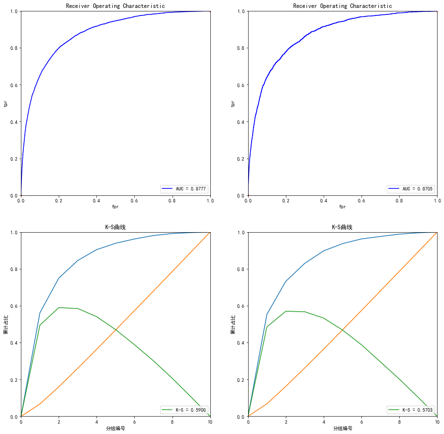
最后训练集，测试集的auc如下：

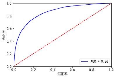
 结果都是差不多，0.8585906092953097

效果还是不错了

2021.01.20更新

本次缺点：没有进行变量挑选，全部都入模了

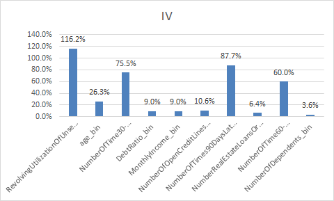
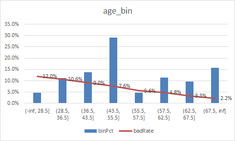
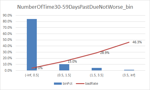
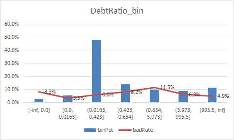
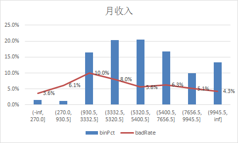
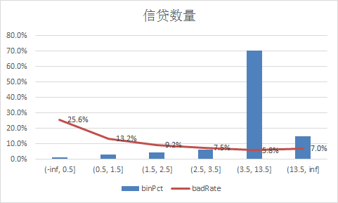
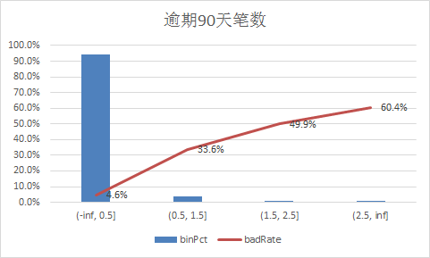
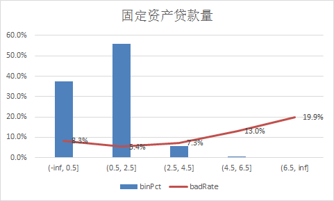
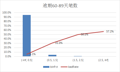
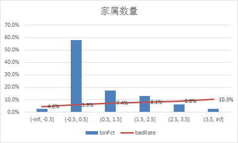
下面补充一下每个变量的iv情况，以及逾期率

 

 

 

 

二、使用逻辑回归模型

首先是前期的处理

# -*- coding: utf-8 -*-
"""
Created on Tue Mar 16 09:40:03 2021

@author: Administrator
"""

#%%导入模块
import pandas as pd 
import numpy as np
from scipy import stats
import seaborn as sns
import matplotlib.pyplot as plt
%matplotlib inline
plt.rc("font",family="SimHei",size="12")  #解决中文无法显示的问题

#%%导入数据
train=pd.read_csv('D:python_homeGive-me-some-credit-masterdata\cs-training.csv')

train.shape  #(150000, 12)
train.pop('Unnamed: 0')

train_copy = train.copy()
train_copy.NumberOfDependents[train_copy.NumberOfDependents.isnull()] = -1
train_copy.MonthlyIncome.median()
train_copy.MonthlyIncome[train_copy.MonthlyIncome.isnull()] = 5400.0


#有iv的计算可知 (35.892, inf]    RevolvingUtilizationOfUnsecuredLines，有点问题，删除
train_copy = train_copy[train_copy.RevolvingUtilizationOfUnsecuredLines<=35.892]
train_copy.shape

#%%分箱
num_iv_woedf = pc.WoeDf()
clf = pc.NumBin(min_bin_samples=200, min_impurity_decrease=4e-5)
for i in ['RevolvingUtilizationOfUnsecuredLines',
       'age', 'NumberOfTime30-59DaysPastDueNotWorse', 'DebtRatio',
       'MonthlyIncome', 'NumberOfOpenCreditLinesAndLoans',
       'NumberOfTimes90DaysLate', 'NumberRealEstateLoansOrLines',
       'NumberOfTime60-89DaysPastDueNotWorse', 'NumberOfDependents']:
    clf.fit(train_copy[i] ,train_copy.SeriousDlqin2yrs)
    train_copy[i+'_bin'] = clf.transform(train_copy[i])  #这样可以省略掉后面转换成_bin的一步骤
    num_iv_woedf.append(clf.woe_df_)
    

#%%woe转换
bin_col = [i for i in list(train_copy.columns) if i[-4:]=='_bin']

cate_iv_woedf = pc.WoeDf()
for i in bin_col:
    cate_iv_woedf.append(pc.cross_woe(train_copy[i] ,train_copy.SeriousDlqin2yrs))
#cate_iv_woedf.to_excel('tmp1')
cate_iv_woedf.bin2woe(train_copy,bin_col)


#%%
model_col = [i for i in list(train_copy.columns) if i[-4:]=='_woe']
x = train_copy[model_col]
y = train_copy[['SeriousDlqin2yrs']]
y.columns = ['y']

#%%建模
import pandas as pd
import matplotlib.pyplot as plt #导入图像库
import matplotlib
import seaborn as sns
import statsmodels.api as sm
from sklearn.metrics import roc_curve, auc
from sklearn.model_selection import train_test_split

x_train,x_test,y_train,y_test=train_test_split(x,y,test_size=0.3,random_state=100)

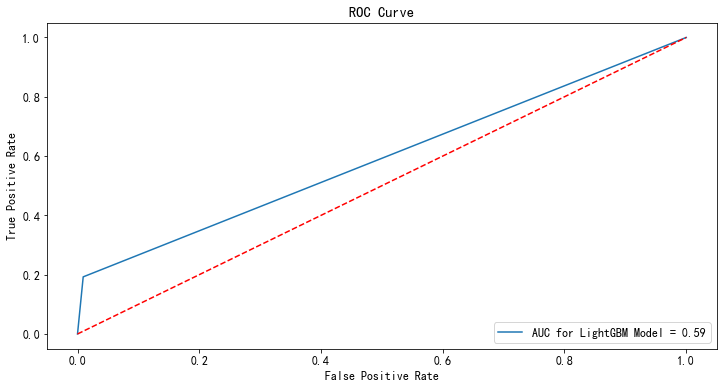
1.逻辑回归不设置参数，即是使用默认的参数

from sklearn.linear_model import LogisticRegression
clf = LogisticRegression()
clf.fit(x_train,y_train)

#用测试集进行检验
p_test = clf.predict(x_test)

fpr,tpr,_ = roc_curve(y_test,p_test)
rocAuc = auc(fpr, tpr)  #0.5917867782621995
plt.figure(figsize=(12,6))
plt.title('ROC Curve')
sns.lineplot(fpr, tpr, label = 'AUC for LightGBM Model = %0.2f' % rocAuc)
plt.legend(loc = 'lower right')
plt.plot([0, 1], [0, 1],'r--')
plt.ylabel('True Positive Rate')
plt.xlabel('False Positive Rate')
plt.show()

 2.我们又使用第一种模型statsmodels

#%%这个是使用 statsmodels
import statsmodels.api as sm
X1=sm.add_constant(x_train)   #在X前加上一列常数1，方便做带截距项的回归
logit=sm.Logit(y_train.astype(float),X1.astype(float))
result=logit.fit()
result.summary()
result.params


#验证集 
X3 = sm.add_constant(x_test)
resu = result.predict(X3.astype(float))
fpr, tpr, threshold = roc_curve(y_test, resu)
rocauc = auc(fpr, tpr)  # 0.8581062561817331
plt.plot(fpr, tpr, 'b', label='AUC = %0.2f' % rocauc)
plt.legend(loc='lower right')
plt.plot([0, 1], [0, 1], 'r--')
plt.xlim([0, 1])
plt.ylim([0, 1])
plt.ylabel('真正率')
plt.xlabel('假正率')
plt.show()

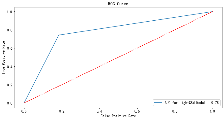
 我们知道逻辑回归默认参数处理不均衡数据效果会很惨，因此设置class_weight="balanced"，

from sklearn.linear_model import LogisticRegression
clf = LogisticRegression(random_state=2021, class_weight="balanced")
clf.fit(x_train,y_train)

#用测试集进行检验
p_test = clf.predict(x_test)

fpr,tpr,_ = roc_curve(y_test,p_test)
rocAuc = auc(fpr, tpr)  #0.7793665739481085
plt.figure(figsize=(12,6))
plt.title('ROC Curve')
sns.lineplot(fpr, tpr, label = 'AUC for LightGBM Model = %0.2f' % rocAuc)
plt.legend(loc = 'lower right')
plt.plot([0, 1], [0, 1],'r--')
plt.ylabel('True Positive Rate')
plt.xlabel('False Positive Rate')
plt.show()

 我们知道class_weight还有另外一种设置方法，但是貌似效果更加差

from sklearn.linear_model import LogisticRegression
clf = LogisticRegression(random_state=2021, class_weight={0:0.93, 1:0.07})
clf.fit(x_train,y_train)

#用测试集进行检验
p_test = clf.predict(x_test)

fpr,tpr,_ = roc_curve(y_test,p_test)
rocAuc = auc(fpr, tpr)  #0.5003326679973387
plt.figure(figsize=(12,6))
plt.title('ROC Curve')
sns.lineplot(fpr, tpr, label = 'AUC for LightGBM Model = %0.2f' % rocAuc)
plt.legend(loc = 'lower right')
plt.plot([0, 1], [0, 1],'r--')
plt.ylabel('True Positive Rate')
plt.xlabel('False Positive Rate')
plt.show()

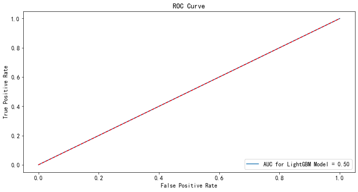
 效果真不好，原因是sklearn的逻辑回归对于这种数据不均衡的样本处理能力会弱一点

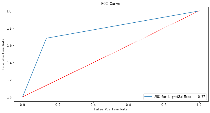
 为了不使用woe转化，我们直接使用lgm建模

# -*- coding: utf-8 -*-
"""
Created on Thu Jan 21 11:28:35 2021

@author: Administrator
"""

#%%该版本直接使用lgb
#%%导入模块
import pandas as pd 
import numpy as np
from scipy import stats
import seaborn as sns
import matplotlib.pyplot as plt
%matplotlib inline
plt.rc("font",family="SimHei",size="12")  #解决中文无法显示的问题

#%%导入数据
train=pd.read_csv('D:python_homeGive-me-some-credit-masterdata\cs-training.csv')
train.pop('Unnamed: 0')

train_copy = train.copy()
train_copy.NumberOfDependents[train_copy.NumberOfDependents.isnull()] = -1
train_copy.MonthlyIncome.median()
train_copy.MonthlyIncome[train_copy.MonthlyIncome.isnull()] = 5400.0


#%%划分数据集
from sklearn import preprocessing
from sklearn import metrics
from sklearn import model_selection
from sklearn import ensemble
from sklearn import tree
from sklearn import linear_model
import os, datetime, sys, random, time
import seaborn as sns
import xgboost as xgs
import lightgbm as lgb

model_col = list(train_copy.columns)
model_col.remove('SeriousDlqin2yrs')

X = train_copy[model_col]
Y = train_copy['SeriousDlqin2yrs']


x_train,x_test,y_train,y_test=train_test_split(X,Y,test_size=0.3,random_state=100)


#%%lgb建模
lgbAttributes = lgb.LGBMClassifier(objective='binary', n_jobs=-1, random_state=100, importance_type='gain')

lgbParameters = {
    'max_depth' : [2,3,4,5],
    'learning_rate': [0.05, 0.1,0.125,0.15],
    'colsample_bytree' : [0.2,0.4,0.6,0.8,1],
    'n_estimators' : [400,500,600,700,800,900],
    'min_split_gain' : [0.15,0.20,0.25,0.3,0.35], #equivalent to gamma in XGBoost
    'subsample': [0.6,0.7,0.8,0.9,1],
    'min_child_weight': [6,7,8,9,10],
    'scale_pos_weight': [10,15,20],
    'min_data_in_leaf' : [100,200,300,400,500,600,700,800,900],
    'num_leaves' : [20,30,40,50,60,70,80,90,100]
}

lgbModel = model_selection.RandomizedSearchCV(lgbAttributes, param_distributions = lgbParameters, cv = 5, random_state=100)

lgbModel.fit(x_train,y_train,feature_name=model_col)

#最佳参数
bestEstimatorLGB = lgbModel.best_estimator_
bestEstimatorLGB

#使用最佳参数建模

bestEstimatorLGB = lgb.LGBMClassifier(colsample_bytree=1, importance_type='gain', learning_rate=0.125,
               max_depth=5, min_child_weight=6, min_data_in_leaf=500,
               min_split_gain=0.3, n_estimators=500, num_leaves=60,
               objective='binary', random_state=100, scale_pos_weight=10,
               subsample=0.7).fit(x_train,y_train,feature_name=model_col)
yPredLGB = bestEstimatorLGB.predict_proba(x_test)
yPredLGB = yPredLGB[:,1]
yTestPredLGB = bestEstimatorLGB.predict(x_test)
print(metrics.classification_report(y_test,yTestPredLGB))

#画图
fpr,tpr,_ = metrics.roc_curve(y_test,yTestPredLGB)
rocAuc = metrics.auc(fpr, tpr)
plt.figure(figsize=(12,6))
plt.title('ROC Curve')
sns.lineplot(fpr, tpr, label = 'AUC for LightGBM Model = %0.2f' % rocAuc)
plt.legend(loc = 'lower right')
plt.plot([0, 1], [0, 1],'r--')
plt.ylabel('True Positive Rate')
plt.xlabel('False Positive Rate')
plt.show()

最后结果

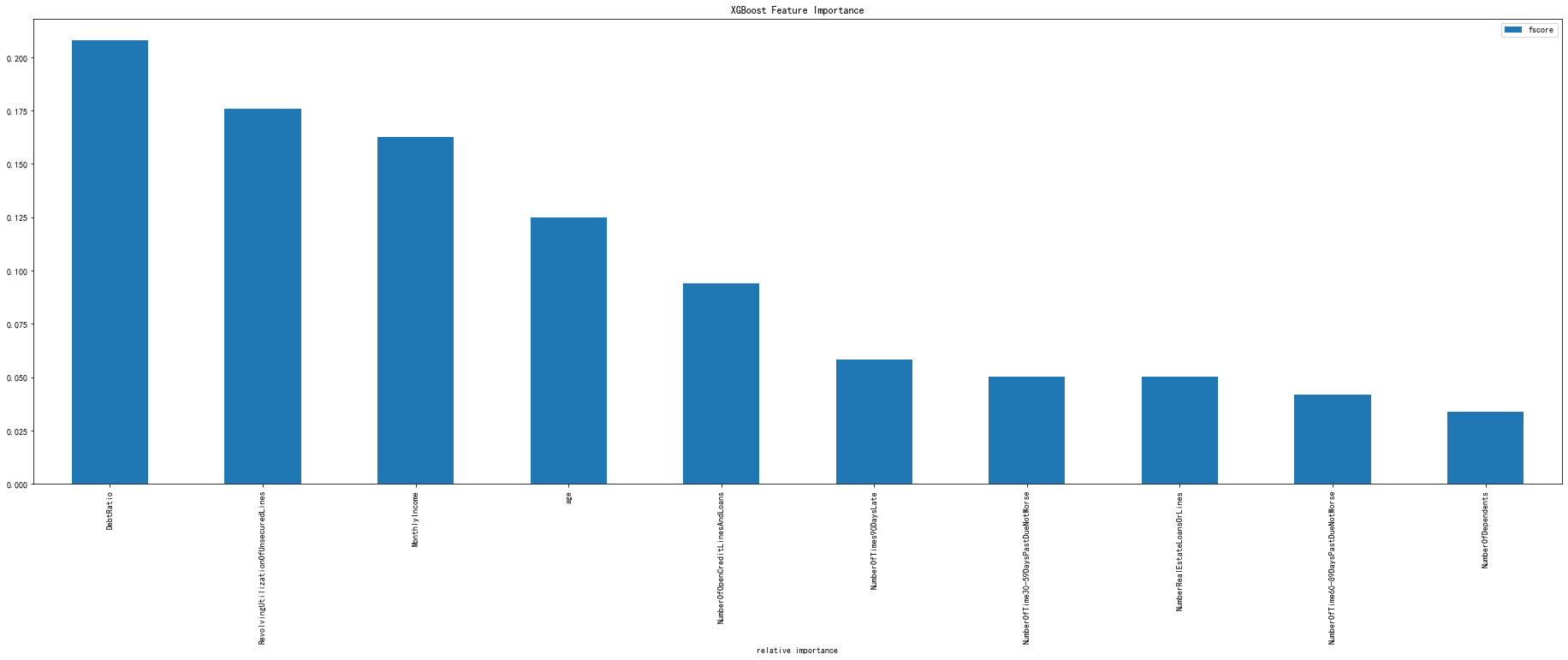
 2021.03.15补充xgboost建模的

# -*- coding: utf-8 -*-
"""
Created on Wed Jan 20 19:33:13 2021

@author: Administrator
"""

#%%导入模块
import pandas as pd 
import numpy as np
from scipy import stats
import seaborn as sns
import matplotlib.pyplot as plt
%matplotlib inline
plt.rc("font",family="SimHei",size="12")  #解决中文无法显示的问题

#%%导入数据
train=pd.read_csv('D:python_homeGive-me-some-credit-masterdata\cs-training.csv')

train.shape  #(150000, 12)
train.pop('Unnamed: 0')
train.columns
'''
[ 'SeriousDlqin2yrs',
       'RevolvingUtilizationOfUnsecuredLines', 'age',
       'NumberOfTime30-59DaysPastDueNotWorse', 'DebtRatio', 'MonthlyIncome',
       'NumberOfOpenCreditLinesAndLoans', 'NumberOfTimes90DaysLate',
       'NumberRealEstateLoansOrLines', 'NumberOfTime60-89DaysPastDueNotWorse',
       'NumberOfDependents']

        {'Unnamed: 0':'id',
        'SeriousDlqin2yrs':'好坏客户',
        'RevolvingUtilizationOfUnsecuredLines':'可用额度比值',
        'age':'年龄',
        'NumberOfTime30-59DaysPastDueNotWorse':'逾期30-59天笔数',
        'DebtRatio':'负债率',
        'MonthlyIncome':'月收入',
        'NumberOfOpenCreditLinesAndLoans':'信贷数量',
        'NumberOfTimes90DaysLate':'逾期90天笔数',
        'NumberRealEstateLoansOrLines':'固定资产贷款量',
        'NumberOfTime60-89DaysPastDueNotWorse':'逾期60-89天笔数',
        'NumberOfDependents':'家属数量'}
'''


#%%查看每个变量的唯一值
for i in list(train.columns):
    print(i,'的唯一值是：',train[i].nunique())
    
'''
SeriousDlqin2yrs 的唯一值是： 2
RevolvingUtilizationOfUnsecuredLines 的唯一值是： 125728
age 的唯一值是： 86
NumberOfTime30-59DaysPastDueNotWorse 的唯一值是： 16
DebtRatio 的唯一值是： 114194
MonthlyIncome 的唯一值是： 13594
NumberOfOpenCreditLinesAndLoans 的唯一值是： 58
NumberOfTimes90DaysLate 的唯一值是： 19
NumberRealEstateLoansOrLines 的唯一值是： 28
NumberOfTime60-89DaysPastDueNotWorse 的唯一值是： 13
NumberOfDependents 的唯一值是： 13
'''
#%%查看缺失值
train.isnull().sum()
'''
SeriousDlqin2yrs                            0
RevolvingUtilizationOfUnsecuredLines        0
age                                         0
NumberOfTime30-59DaysPastDueNotWorse        0
DebtRatio                                   0
MonthlyIncome                           29731
NumberOfOpenCreditLinesAndLoans             0
NumberOfTimes90DaysLate                     0
NumberRealEstateLoansOrLines                0
NumberOfTime60-89DaysPastDueNotWorse        0
NumberOfDependents                       3924
dtype: int64
'''
#月收入缺失比例还是很高的，展示不管
#%%按照字面理解。好像都是数值型变量
import pycard as pc
num_iv_woedf = pc.WoeDf()
clf = pc.NumBin()
for i in list(train.columns):
    clf.fit(train[i] ,train.SeriousDlqin2yrs)
    clf.generate_transform_fun()
    num_iv_woedf.append(clf.woe_df_)
num_iv_woedf.to_excel('tmp18')


#上面可知有2个字段是有缺失值得，我们可以将NumberOfDependents填补为-1，收入的填补为均值
train_copy = train.copy()
train_copy.NumberOfDependents[train_copy.NumberOfDependents.isnull()] = -1
train_copy.MonthlyIncome.median()
train_copy.MonthlyIncome[train_copy.MonthlyIncome.isnull()] = 5400.0


#有iv的计算可知 (35.892, inf]    RevolvingUtilizationOfUnsecuredLines，有点问题，删除
train_copy = train_copy[train_copy.RevolvingUtilizationOfUnsecuredLines<=35.892]
train_copy.shape


#%%异常值处理
#我错了，下面这个异常值处理并不合理，不处理了，

#%%分箱
import pycard as pc
num_iv_woedf = pc.WoeDf()
clf = pc.NumBin()
for i in list(train_copy.columns)[1:]:
    clf.fit(train_copy[i] ,train_copy.SeriousDlqin2yrs)
    clf.generate_transform_fun()
    num_iv_woedf.append(clf.woe_df_)





from numpy import *
train_copy['RevolvingUtilizationOfUnsecuredLines_bin'] = pd.cut(train_copy.RevolvingUtilizationOfUnsecuredLines,bins=[-inf, 0.1318, 0.3009, 0.495, 0.6981, 0.8628, 1.0051, 1.0284, inf])
train_copy['age_bin'] = pd.cut(train_copy.age,bins=[-inf, 28.5, 36.5, 43.5, 55.5, 57.5, 62.5, 67.5, inf])
train_copy['NumberOfTime30-59DaysPastDueNotWorse_bin'] = pd.cut(train_copy['NumberOfTime30-59DaysPastDueNotWorse'],bins=[-inf, 0.5, 1.5, 3.5, inf])
train_copy['DebtRatio_bin'] = pd.cut(train_copy.DebtRatio,bins=[-inf, 0.0, 0.0163, 0.4233, 0.6537, 3.9728, 995.5, inf])
train_copy['MonthlyIncome_bin'] = pd.cut(train_copy.MonthlyIncome,bins=[-inf, 270.0, 930.5, 3332.5, 5320.5, 5400.5, 7656.5, 9945.5, inf])
train_copy['NumberOfOpenCreditLinesAndLoans_bin'] = pd.cut(train_copy.NumberOfOpenCreditLinesAndLoans,bins=[-inf, 0.5, 1.5, 2.5, 3.5, 13.5, inf])
train_copy['NumberOfTimes90DaysLate_bin'] = pd.cut(train_copy.NumberOfTimes90DaysLate,bins=[-inf, 0.5, 1.5, 2.5, inf])
train_copy['NumberRealEstateLoansOrLines_bin'] = pd.cut(train_copy.NumberRealEstateLoansOrLines,bins=[-inf, 0.5, 2.5, 4.5, 6.5, inf])
train_copy['NumberOfTime60-89DaysPastDueNotWorse_bin'] = pd.cut(train_copy['NumberOfTime60-89DaysPastDueNotWorse'],bins=[-inf, 0.5, 1.5, 2.5, inf])
train_copy['NumberOfDependents_bin'] = pd.cut(train_copy.NumberOfDependents,bins=[-inf, -0.5, 0.5, 1.5, 2.5, 3.5, inf])


cate_iv_woedf = pc.WoeDf()
clf = pc.NumBin()
for i in ['RevolvingUtilizationOfUnsecuredLines_bin',
       'age_bin', 'NumberOfTime30-59DaysPastDueNotWorse_bin', 'DebtRatio_bin',
       'MonthlyIncome_bin', 'NumberOfOpenCreditLinesAndLoans_bin',
       'NumberOfTimes90DaysLate_bin', 'NumberRealEstateLoansOrLines_bin',
       'NumberOfTime60-89DaysPastDueNotWorse_bin', 'NumberOfDependents_bin']:
    cate_iv_woedf.append(pc.cross_woe(train_copy[i] ,train_copy.SeriousDlqin2yrs))
cate_iv_woedf.to_excel('tmp18')


#%%woe转换
iv_col = ['RevolvingUtilizationOfUnsecuredLines_bin',
       'age_bin', 'NumberOfTime30-59DaysPastDueNotWorse_bin', 'DebtRatio_bin',
       'MonthlyIncome_bin', 'NumberOfOpenCreditLinesAndLoans_bin',
       'NumberOfTimes90DaysLate_bin', 'NumberRealEstateLoansOrLines_bin',
       'NumberOfTime60-89DaysPastDueNotWorse_bin', 'NumberOfDependents_bin']
cate_iv_woedf.bin2woe(train_copy,iv_col)

model_col = [i for i in ['SeriousDlqin2yrs']+list(train_copy.columns)[-10:]]

#%%建模
import pandas as pd
import matplotlib.pyplot as plt #导入图像库
import matplotlib
import seaborn as sns
import statsmodels.api as sm
from sklearn.metrics import roc_curve, auc
from sklearn.model_selection import train_test_split

X = train_copy[model_col[1:]]
Y = train_copy['SeriousDlqin2yrs']


x_train,x_test,y_train,y_test=train_test_split(X,Y,test_size=0.3,random_state=100)

#(10127, 44)

X1=sm.add_constant(x_train)   #在X前加上一列常数1，方便做带截距项的回归
logit=sm.Logit(y_train.astype(float),X1.astype(float))
result=logit.fit()
result.summary()
result.params


#验证集 
X3 = sm.add_constant(x_test)
resu = result.predict(X3.astype(float))
fpr, tpr, threshold = roc_curve(y_test, resu)
rocauc = auc(fpr, tpr)  # 0.8575936062678856
plt.plot(fpr, tpr, 'b', label='AUC = %0.2f' % rocauc)
plt.legend(loc='lower right')
plt.plot([0, 1], [0, 1], 'r--')
plt.xlim([0, 1])
plt.ylim([0, 1])
plt.ylabel('真正率')
plt.xlabel('假正率')
plt.show()

#训练集
resu_1 = result.predict(X1.astype(float))
fpr, tpr, threshold = roc_curve(y_train, resu_1)
rocauc = auc(fpr, tpr)  #0.8585906092953097
plt.plot(fpr, tpr, 'b', label='AUC = %0.2f' % rocauc)
plt.legend(loc='lower right')
plt.plot([0, 1], [0, 1], 'r--')
plt.xlim([0, 1])
plt.ylim([0, 1])
plt.ylabel('真正率')
plt.xlabel('假正率')
plt.show()


#%%测试集
test = pd.read_csv('D:python_homeGive-me-some-credit-masterdata\cs-test.csv')


test.NumberOfDependents[test.NumberOfDependents.isnull()] = -1
test.MonthlyIncome.median()
test.MonthlyIncome[test.MonthlyIncome.isnull()] = 5400.0

test['RevolvingUtilizationOfUnsecuredLines_bin'] = pd.cut(test.RevolvingUtilizationOfUnsecuredLines,bins=[-inf, 0.1318, 0.3009, 0.495, 0.6981, 0.8628, 1.0051, 1.0284, inf])
test['age_bin'] = pd.cut(test.age,bins=[-inf, 28.5, 36.5, 43.5, 55.5, 57.5, 62.5, 67.5, inf])
test['NumberOfTime30-59DaysPastDueNotWorse_bin'] = pd.cut(test['NumberOfTime30-59DaysPastDueNotWorse'],bins=[-inf, 0.5, 1.5, 3.5, inf])
test['DebtRatio_bin'] = pd.cut(test.DebtRatio,bins=[-inf, 0.0, 0.0163, 0.4233, 0.6537, 3.9728, 995.5, inf])
test['MonthlyIncome_bin'] = pd.cut(test.MonthlyIncome,bins=[-inf, 270.0, 930.5, 3332.5, 5320.5, 5400.5, 7656.5, 9945.5, inf])
test['NumberOfOpenCreditLinesAndLoans_bin'] = pd.cut(test.NumberOfOpenCreditLinesAndLoans,bins=[-inf, 0.5, 1.5, 2.5, 3.5, 13.5, inf])
test['NumberOfTimes90DaysLate_bin'] = pd.cut(test.NumberOfTimes90DaysLate,bins=[-inf, 0.5, 1.5, 2.5, inf])
test['NumberRealEstateLoansOrLines_bin'] = pd.cut(test.NumberRealEstateLoansOrLines,bins=[-inf, 0.5, 2.5, 4.5, 6.5, inf])
test['NumberOfTime60-89DaysPastDueNotWorse_bin'] = pd.cut(test['NumberOfTime60-89DaysPastDueNotWorse'],bins=[-inf, 0.5, 1.5, 2.5, inf])
test['NumberOfDependents_bin'] = pd.cut(test.NumberOfDependents,bins=[-inf, -0.5, 0.5, 1.5, 2.5, 3.5, inf])


cate_iv_woedf.bin2woe(test,iv_col)

X_test = test[model_col[1:]]
X4 = sm.add_constant(X_test.astype(float))
resu_test = result.predict(X4.astype(float))

至于后面为什么没有将调参进行到第五步，那是因为后面的效果比前面的还要差，我们就不继续进行了。

补充一些代码

train_x, test_x, train_y, test_y = train_test_split(train_x.values, train_y.values, test_size=0.25, random_state=1234)
plot_roc(test_x, test_y)

 

 如果我们没有那么多时间去调参，我们可以直接使用这个模板

#%%
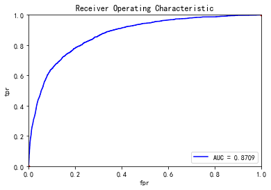
import pandas as pd
import xgboost as xgb
from sklearn.model_selection import train_test_split
from sklearn.externals import joblib
import logging

train=pd.read_csv('D:python_homeGive-me-some-credit-masterdata\cs-training.csv')
train.pop('Unnamed: 0')


data_y = train[['SeriousDlqin2yrs']]
data_y.columns = ['y']
data_x = train.drop(['SeriousDlqin2yrs'],axis=1)


train_x, test_x, train_y, test_y = train_test_split(data_x.values, data_y.values, test_size=0.2,random_state=1234)
d_train = xgb.DMatrix(train_x, label=train_y)
d_valid = xgb.DMatrix(test_x, label=test_y)
watchlist = [(d_train, 'train'), (d_valid, 'valid')]
#参数设置
params={
    'eta': 0.2, # 特征权重 取值范围0~1 通常最后设置eta为0.01~0.2
    'max_depth':3,   # 通常取值：3-10 树的深度
    'min_child_weight':6, # 最小样本的权重，调大参数可以防止过拟合
    'gamma':0.3,
    'subsample':0.8, #随机取样比例
    'colsample_bytree':0.8, #默认为1 ，取值0~1 对特征随机采集比例
    'booster':'gbtree', #迭代树
    'objective': 'binary:logistic', #逻辑回归，输出为概率
    'nthread':8, #设置最大的进程量，若不设置则会使用全部资源
    'scale_pos_weight': 10, #默认为0，1可以处理类别不平衡
    'lambda':1,   #默认为1
    'seed':1234, #随机数种子
    'silent':1 , #0表示输出结果
    'eval_metric': 'auc' # 检验指标
}
bst = xgb.train(params, d_train,1000,watchlist,early_stopping_rounds=500, verbose_eval=10)
tree_nums=bst.best_ntree_limit
print('最优模型树的数量：%s，auc：%s' % (bst.best_ntree_limit, bst.best_score)) #最优模型树的数量：81，auc：0.870911
bst = xgb.train(params, d_train,tree_nums,watchlist,early_stopping_rounds=500, verbose_eval=10)
#joblib.dump(bst, 'd:/xgboost.model') #保存模型

plot_roc(test_x, test_y)

其中画roc还是使用上面的函数