HashMap 是 Map 基于哈希散列算法的实现,其在 JDK1.7 中采用了数组+链表的数据结构。在 JDK1.8 中为了提高查询效率,采用了数组+链表+红黑树的数据结构。本文所有讲解均基于 JDK1.8 进行讲解。
public class HashMap<K,V> extends AbstractMap<K,V>
    implements Map<K,V>, Cloneable, Serializable
从上面 HashMap 的定义可以看出,其继承了 AbstractMap,实现了 Map 接口。
原理
我们将从类成员变量、构造方法、核心方法、扩容机制几个方向介绍 HashMap 的原理。
类成员变量
// 默认大小
static final int DEFAULT_INITIAL_CAPACITY = 1 << 4; // aka 16
// 最大大小
static final int MAXIMUM_CAPACITY = 1 << 30;
// 默认扩展因子
static final float DEFAULT_LOAD_FACTOR = 0.75f;
// 树化阈值。当超过这个阈值时,链表转成红黑树。
static final int TREEIFY_THRESHOLD = 8;
// 链化阈值。当低于这个阈值时,红黑树转成链表。
static final int UNTREEIFY_THRESHOLD = 6;
// 允许树化的最小容量。只有容量超过此值时,才允许进行树化操作。
static final int MIN_TREEIFY_CAPACITY = 64;
// 桶数组
transient Node<K,V>[] table;
// 大小
transient int size;
// 调整阈值
int threshold;
// 扩展因子
final float loadFactor;
// 省略其他不重要的变量
在上面的类成员变量中,最重要的是 table 这个变量,其实一个 Node 类型的数组。我们知道 HashMap 是一个数组 + 链表 + 红黑树的结构,其示意图如下所示:
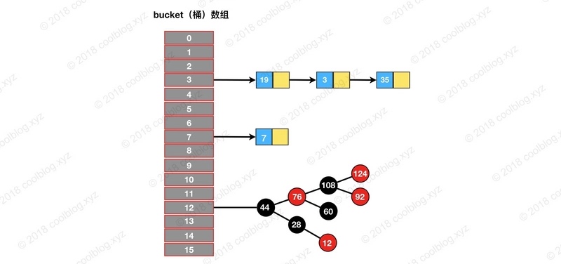
这里的 table 数组就相当于上图中的 bucket 数组,而每个数组下标都对应着一个个的 Node 节点。这个 Node 节点可能是链表节点,也可能是红黑树节点。说到 Node 节点,我们有必要详细说说 Node 节点的类关系图。
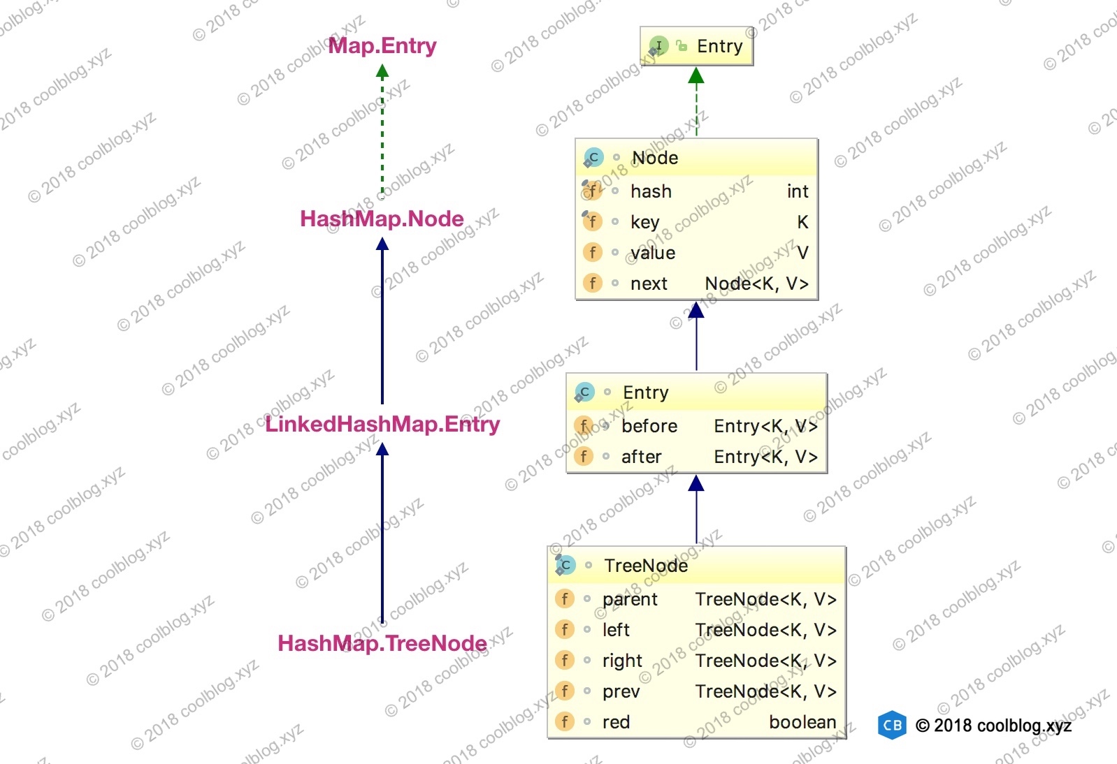
在上面的类关系图中,最上层是 Map.Entry 接口,其是一条数据的抽象化,有 key 和 value 各种操作。接着,HashMap.Node 实现了 Map.Entry 接口,并且增加了 hash、key、value、next 等属性,表示其是一个哈希节点。接着,LinkedHashMap.Entry 继承了 HashMap.Node 节点,并且增加了 before、after 节点用来存储元素的插入顺序,表示其实一个维护着插入顺序的链表哈希节点。最后,HashMap.TreeNode 继承了 LinkedHashMap.Entry,并且增加了 parent、left、right、prev、red 节点用来存储红黑树相关信息,表示其实一个红黑树的节点。但因为其继承自 LinkedHashMap.Entry,所以其也维护了插入元素的顺序。
看完 Node 节点的类关系图,我们再来看 HashMap 中定义的 Node 类型 table 数组。我们会发现这个 Node 类型,其实就是 HashMap.Node。如果该桶是链表,那么插入的是 HashMap.Node 对象。如果是红黑树,那么插入的是 HashMap.TreeNode 对象。
构造方法
HashMap 一共有 4 个构造方法。
public HashMap() {
    this.loadFactor = DEFAULT_LOAD_FACTOR;
}

public HashMap(int initialCapacity) {
    this(initialCapacity, DEFAULT_LOAD_FACTOR);
}

public HashMap(int initialCapacity, float loadFactor) {
    if (initialCapacity < 0)
        throw new IllegalArgumentException("Illegal initial capacity: " + initialCapacity);
    if (initialCapacity > MAXIMUM_CAPACITY)
        initialCapacity = MAXIMUM_CAPACITY;
    if (loadFactor <= 0 || Float.isNaN(loadFactor))
        throw new IllegalArgumentException("Illegal load factor: " +
                                           loadFactor);
    this.loadFactor = loadFactor;
    this.threshold = tableSizeFor(initialCapacity);
}

public HashMap(Map<? extends K, ? extends V> m) {
    this.loadFactor = DEFAULT_LOAD_FACTOR;
    putMapEntries(m, false);
}
上面这几个构造方法中,比较值得注意的是第 3 个构造方法。其中有这个一行代码:
this.threshold = tableSizeFor(initialCapacity);
从上面的代码我们可以看到:其调用了 tableSizeFor 方法,并将 initialCapacity 作为参数传入,最后将返回值设置给了 this.threshold。我们先看看 tableSizeFor 方法。
static final int tableSizeFor(int cap) {
    int n = cap - 1;
    n |= n >>> 1;
    n |= n >>> 2;
    n |= n >>> 4;
    n |= n >>> 8;
    n |= n >>> 16;
    return (n < 0) ? 1 : (n >= MAXIMUM_CAPACITY) ? MAXIMUM_CAPACITY : n + 1;
}
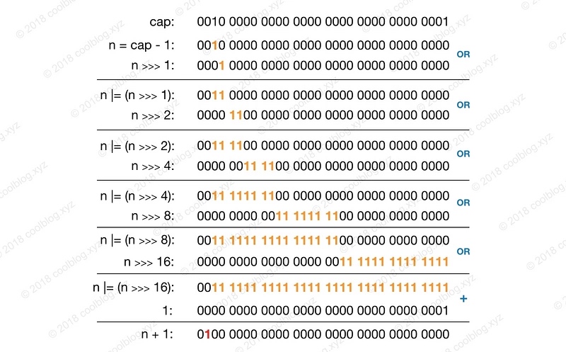
简单地说,tableSizeFor 的用途是:找到大于或等于 cap 的最小2的幂。具体的计算过程可以参考下图。
最后我们回到刚刚的那个构造方法:
public HashMap(int initialCapacity, float loadFactor) {
    if (initialCapacity < 0)
        throw new IllegalArgumentException("Illegal initial capacity: " + initialCapacity);
    if (initialCapacity > MAXIMUM_CAPACITY)
        initialCapacity = MAXIMUM_CAPACITY;
    if (loadFactor <= 0 || Float.isNaN(loadFactor))
        throw new IllegalArgumentException("Illegal load factor: " +
                                           loadFactor);
    this.loadFactor = loadFactor;
    this.threshold = tableSizeFor(initialCapacity);
}
我们仔细看就会发现,虽然我们传入了 initialCapacity,但是貌似没有进行数据初始化工作呀。没错,HashMap 在创建的时候并不会进行数据的初始化,而是在真正插入的时候才进行初始化操作。这一部分的代码在 resize (扩容)方法中,我们后续会讲到。
核心方法
对于 HashMap 来说,作为核心的几个方法为:get、put、remove。
get
HashMap 的查找操作比较简单,首先定位键值对所在桶的位置,之后再对链表或红黑树进行查找。
public V get(Object key) {
    Node<K,V> e;
    return (e = getNode(hash(key), key)) == null ? null : e.value;
}

final Node<K,V> getNode(int hash, Object key) {
    Node<K,V>[] tab; Node<K,V> first, e; int n; K k;
    // 1.桶不为空,那么进行查找,否则直接返回 null。
    if ((tab = table) != null && (n = tab.length) > 0 &&
        (first = tab[(n - 1) & hash]) != null) {
        // 1.1 检查要查找的是否是第一个节点
        if (first.hash == hash && // always check first node
            ((k = first.key) == key || (key != null && key.equals(k))))
            return first;
        // 1.2 沿着第一个节点继续查找
        if ((e = first.next) != null) {
            // 1.2.1 如果是红黑树,那么调用红黑树的方法查找
            if (first instanceof TreeNode)
                return ((TreeNode<K,V>)first).getTreeNode(hash, key);
            // 1.2.2 如果是链表,那么采用链表的方式查找
            do {
                if (e.hash == hash &&
                    ((k = e.key) == key || (key != null && key.equals(k))))
                    return e;
            } while ((e = e.next) != null);
        }
    }
    return null;
}
上面的逻辑其实不难看懂。但在上面计算 key 所在桶位置时,我们采用的是与运算,而不是取余操作。
first = tab[(n - 1) & hash]) != null
HashMap 中的桶数组大小总是为 2 的幂。在这个情况下,(n - 1) & hash 等价于对 length 取余。但取余的计算效率没有位运算高,所以(n - 1) & hash也是一个小的优化。
另外,在计算哈希值的时候,我们会发现 hash 方法并不是直接用 key.hashCode 方法产生的哈希值,而是做了一些位操作。
/**
 * 计算键的 hash 值
 */
static final int hash(Object key) {
    int h;
    return (key == null) ? 0 : (h = key.hashCode()) ^ (h >>> 16);
}
看这个方法的逻辑好像是通过位运算重新计算 hash,那么这里为什么要这样做呢?为什么不直接用键的 hashCode 方法产生的 hash 呢?
在上面的讲解我们知道,我们最终会用 n - 1 和 hash 进行与运算,就像下面这样。

但很多时候我们的 n(桶大小)都比较小,也就是说 n - 1 非常小。这样就会导致做与操作时,无论 hash 值的高 4 位是什么值,n - 1 & hash 的值的高四位都为 0。也就是说hash 只有低4位参与了计算,高位的计算可以认为是无效的。这样会导致哈希出来的值只受 hash 低 4 位的影响,大大增加哈希碰撞的概率。
而 hash 方法中的 (h = key.hashCode()) ^ (h >>> 16) 其实是将 hash 值的高 16 位于低 16 位进行一次异或运算,从而加大低位信息的随机性,变相的让高位数据参与到计算中。此时的计算过程如下:

put
我们先看看 put 方法的实现。
public V put(K key, V value) {
    return putVal(hash(key), key, value, false, true);
}
可以看到 HashMap 的 put 方法其实是调用了 putVal 方法。
final V putVal(int hash, K key, V value, boolean onlyIfAbsent,
               boolean evict) {
    Node<K,V>[] tab; Node<K,V> p; int n, i;
    // 1. 如果未初始化,那么调用 resize() 进行初始化
    if ((tab = table) == null || (n = tab.length) == 0)
        n = (tab = resize()).length;
    // 2. 如果桶为空,那么直接插入
    if ((p = tab[i = (n - 1) & hash]) == null)
        tab[i] = newNode(hash, key, value, null);
    else {
        Node<K,V> e; K k;
        // 2.1 如果插入的元素与桶第一个元素相同,那么直接跳出
        if (p.hash == hash &&
            ((k = p.key) == key || (key != null && key.equals(k))))
            e = p;
        // 2.2 如果第一个元素是红黑树节点,那么调用红黑树的插入方法
        else if (p instanceof TreeNode)
            e = ((TreeNode<K,V>)p).putTreeVal(this, tab, hash, key, value);
        // 2.3 如果是链表节点,那么遍历到链表尾部插入。但如果中间找到了相同的节点,那么直接退出
        else {
            for (int binCount = 0; ; ++binCount) {
                if ((e = p.next) == null) {
                    p.next = newNode(hash, key, value, null);
                    if (binCount >= TREEIFY_THRESHOLD - 1) // -1 for 1st
                        treeifyBin(tab, hash); //判断是否树化
                    break;
                }
                if (e.hash == hash &&
                    ((k = e.key) == key || (key != null && key.equals(k))))
                    break;
                p = e;
            }
        }
        // 3. 如果插入的key已经存在,那么根据参数判断是否替代旧值
        // 这里的 e 如果不为 null,那么就存储着旧值
        if (e != null) { // existing mapping for key
            V oldValue = e.value;
            if (!onlyIfAbsent || oldValue == null)
                e.value = value;
            afterNodeAccess(e);
            return oldValue;
        }
    }
    ++modCount;
    // 4.判断是否扩容
    if (++size > threshold)
        resize();
    afterNodeInsertion(evict);
    return null;
}
上面代码的大致逻辑为:
- 如果桶数组 table 为空,那么通过扩容的方式初始化 table 数组。
- 如果插入的桶为空,那么直接插入。如果插入的桶不为空,那么判断是否与该桶第一个节点相同。如果相同,那么直接退出。否则根据节点不同类型,调用不同的插入方式。如果是红黑树节点,那么调用 putTreeVal 方法。如果是链表节点,那么直接插入链表尾部。在遍历链表的过程中,会判断节点是否存在。如果存在,则会直接跳出循环。
- 根据条件判断 key 是否存在,如果存在则根据参数判断是否替换旧值。
- 最后根据参数判断是否扩容。
remove
HashMap 的删除操作并不复杂,仅需三个步骤即可完成。第一步是定位桶位置,第二步遍历链表并找到键值相等的节点,第三步删除节点。相关源码如下:
public V remove(Object key) {
    Node<K,V> e;
    return (e = removeNode(hash(key), key, null, false, true)) == null ?
        null : e.value;
}

final Node<K,V> removeNode(int hash, Object key, Object value,
                           boolean matchValue, boolean movable) {
    Node<K,V>[] tab; Node<K,V> p; int n, index;
    if ((tab = table) != null && (n = tab.length) > 0 &&
        (p = tab[index = (n - 1) & hash]) != null) {
        Node<K,V> node = null, e; K k; V v;
        // 1. 查找到要删除的节点
        if (p.hash == hash &&
            ((k = p.key) == key || (key != null && key.equals(k))))
            node = p;
        else if ((e = p.next) != null) {
            if (p instanceof TreeNode)
                node = ((TreeNode<K,V>)p).getTreeNode(hash, key);
            else {
                do {
                    if (e.hash == hash &&
                        ((k = e.key) == key ||
                         (key != null && key.equals(k)))) {
                        node = e;
                        break;
                    }
                    p = e;
                } while ((e = e.next) != null);
            }
        }
        // 2. 删除查找到的节点
        if (node != null && (!matchValue || (v = node.value) == value ||
                             (value != null && value.equals(v)))) {
            if (node instanceof TreeNode)
                ((TreeNode<K,V>)node).removeTreeNode(this, tab, movable);
            else if (node == p)
                tab[index] = node.next;
            else
                p.next = node.next;
            ++modCount;
            --size;
            afterNodeRemoval(node);
            return node;
        }
    }
    return null;
}
扩容机制
在 HashMap 中,桶数组的长度均是2的幂,阈值大小为桶数组长度与负载因子的乘积。当 HashMap 中的键值对数量超过阈值时,进行扩容。
HashMap 的扩容机制与其他变长集合的套路不太一样,HashMap 按当前桶数组长度的2倍进行扩容,阈值也变为原来的2倍(如果计算过程中,阈值溢出归零,则按阈值公式重新计算)。扩容之后,要重新计算键值对的位置,并把它们移动到合适的位置上去。以上就是 HashMap 的扩容大致过程,接下来我们来看看具体的实现:
final Node<K,V>[] resize() {
    Node<K,V>[] oldTab = table;
    int oldCap = (oldTab == null) ? 0 : oldTab.length;
    int oldThr = threshold;
    int newCap, newThr = 0;
    // 1.根据不同情况,设置新的容量和阈值
    // 1.1 如果不为空,表示已经初始化了。
    if (oldCap > 0) {
        // 超过最大容量,不再扩容
        if (oldCap >= MAXIMUM_CAPACITY) {
            threshold = Integer.MAX_VALUE;
            return oldTab;
        }
        // 按照旧容量和旧阈值的2倍计算新容量和新阈值
        else if ((newCap = oldCap << 1) < MAXIMUM_CAPACITY &&
                 oldCap >= DEFAULT_INITIAL_CAPACITY)
            newThr = oldThr << 1; // double threshold
    }
    // 1.2 走到这里,表示 oldCap <= 0。如果此时,oldThr > 0,表示有设置了初始值
    // 那么将初始值 oldThr 作为新的容量大小。
    // 注意:我们在初始化时调用 tableForSize 参数,将初始大小存在了threshold中
    // 所以此时 oldThr 就是我们设置的 initCapacity
    else if (oldThr > 0)
        newCap = oldThr;
    else {
    // 1.3 到这里,说明之前没有初始化,也没有设置初始值,那么就按照默认值进行设置
        newCap = DEFAULT_INITIAL_CAPACITY;
        newThr = (int)(DEFAULT_LOAD_FACTOR * DEFAULT_INITIAL_CAPACITY);
    }
    // 2. 如果新的阈值为0,那么就按照阈值计算公式计算
    if (newThr == 0) {
        float ft = (float)newCap * loadFactor;
        newThr = (newCap < MAXIMUM_CAPACITY && ft < (float)MAXIMUM_CAPACITY ?
                  (int)ft : Integer.MAX_VALUE);
    }
    threshold = newThr;
    // 3. 开始复制到新的数组
    @SuppressWarnings({"rawtypes","unchecked"})
        Node<K,V>[] newTab = (Node<K,V>[])new Node[newCap];
    table = newTab;
    if (oldTab != null) {
        // 3.1 循环遍历旧的 table 数组
        for (int j = 0; j < oldCap; ++j) {
            Node<K,V> e;
            if ((e = oldTab[j]) != null) {
                oldTab[j] = null;
                // 3.1.1 如果该桶只有一个元素,那么直接复制
                if (e.next == null)
                    newTab[e.hash & (newCap - 1)] = e;
                // 3.1.2 如果死红黑树,那么对红黑树进行拆分
                else if (e instanceof TreeNode)
                    ((TreeNode<K,V>)e).split(this, newTab, j, oldCap);
                // 3.1.3 遍历链表,将原链表节点分成lo和hi两个链表
                // 其中 lo 表示在原来的桶位置,hi 表示在新的桶位置
                else { // preserve order
                    Node<K,V> loHead = null, loTail = null;
                    Node<K,V> hiHead = null, hiTail = null;
                    Node<K,V> next;
                    do {
                        next = e.next;
                        // 3.1.3.1 hash & oldCap 等于0,表示在原位置
                        if ((e.hash & oldCap) == 0) {
                            if (loTail == null)
                                loHead = e;
                            else
                                loTail.next = e;
                            loTail = e;
                        }
                        // 3.1.3.2 hash & oldCap 不等于0,表示要移位
                        else {
                            if (hiTail == null)
                                hiHead = e;
                            else
                                hiTail.next = e;
                            hiTail = e;
                        }
                    } while ((e = next) != null);
                    // 3.1.3.3 将分组后的链表映射到新桶中
                    if (loTail != null) {
                        loTail.next = null;
                        newTab[j] = loHead;
                    }
                    if (hiTail != null) {
                        hiTail.next = null;
                        newTab[j + oldCap] = hiHead;
                    }
                }
            }
        }
    }
    return newTab;
}
在上面的扩容过程中,最重要的是其怎么将链表拆分到合适的位置上。我们先来看一个例子。
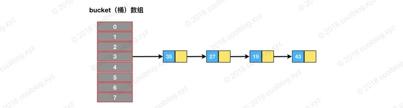
在上面这个例子中,capacity 为 8,在 第 4 个桶上有:35、27、19、43 这四个节点。其扩容前后的计算过程如下:
// 扩容前
100011  // 35
000111  // n-1=8-1=7
000011  // 35&n-1 = 3
// 扩容后
100011  // 35
001111  // n-1=16-1=15
000011  // 35&n-1 = 3
你会发现其扩容前后的值都为 3。我们再来看看 27 这个节点在扩容前和扩容后的计算过程:
// 扩容前
011011  // 27
000111  // n-1=8-1=7
000011  // 27&n-1 = 3
// 扩容后
011011  // 27
001111  // n-1=16-1=15
001011  // 27&n-1 = 11
你会发现 27 这个节点扩容后的桶位置发生了变化。这是因为扩容后,参与模运算的位数由4位变为了5位。由于两个 27 和 35 两个节点第5位的值是不一样,所以两个 hash 算出的结果也不一样。而且其变化后的位置为原来的位置加上第5位的值,也就是 olcCapacity + 原位置(对于本例中的 27 就是:3 + 8 = 11)。
知道了这个规律,那么我们再来看链表分组的代码就简单多了。
Node<K,V> loHead = null, loTail = null;
Node<K,V> hiHead = null, hiTail = null;
Node<K,V> next;
do {
    next = e.next;
    // 3.1.3.1 hash & oldCap 等于0,表示在原位置
    if ((e.hash & oldCap) == 0) {
        if (loTail == null)
            loHead = e;
        else
            loTail.next = e;
        loTail = e;
    }
    // 3.1.3.2 hash & oldCap 不等于0,表示要移位
    else {
        if (hiTail == null)
            hiHead = e;
        else
            hiTail.next = e;
        hiTail = e;
    }
} while ((e = next) != null);
从上面的代码可以看到最外层是一个循环,遍历整个链表。3.1.3.1 就是判断如果是 e.hash & oldCap = 0(即原 hash 值某一位位0,那么其位置就不变),那么就放在 loTail 为首的链表中,这个链表存的是扩容后放置在原来桶位置的节点。而 hiTail 放置的则是要移位到 oldCapacity + 原位置 的链表。
// 3.1.3.3 将分组后的链表映射到新桶中
if (loTail != null) {
    loTail.next = null;
    newTab[j] = loHead;
}
if (hiTail != null) {
    hiTail.next = null;
    newTab[j + oldCap] = hiHead;
}
当处理完成后,我们可以看到其直接将 table 桶指向了 loHead 或 hiHead 节点。
链表树化
当桶中链表长度超过 TREEIFY_THRESHOLD(默认为8)时,就会调用 treeifyBin 方法进行树化操作。但此时并不一定会树化,因为在 treeifyBin 方法中还会判断 HashMap 的容量是否大于等于 64。如果容量大于等于 64,那么进行树化,否则优先进行扩容。
为什么树化还要判断整体容量是否大于 64 呢?
当桶数组容量比较小时,键值对节点 hash 的碰撞率可能会比较高,进而导致链表长度较长,从而导致查询效率低下。这时候我们有两种选择,一种是扩容,让哈希碰撞率低一些。另一种是树化,提高查询效率。
如果我们采用扩容,那么我们需要做的就是做一次链表数据的复制。而如果我们采用树化,那么我们需要将链表转化成红黑树。到这里,貌似没有什么太大的区别,但我们让场景继续延伸下去。当插入的数据越来越多,我们会发现需要转化成树的链表越来越多。
到了一定容量,我们就需要进行扩容了。这个时候我们有许多树化的红黑树,在扩容之时,我们需要将许多的红黑树拆分成链表,这是一个挺大的成本。而如果我们在容量小的时候就进行扩容,那么需要树化的链表就越少,我们扩容的成本也就越低。
接下来我们看看链表树化是怎么做的:
final void treeifyBin(Node<K,V>[] tab, int hash) {
    int n, index; Node<K,V> e;
    // 1. 容量小于 MIN_TREEIFY_CAPACITY,优先扩容
    if (tab == null || (n = tab.length) < MIN_TREEIFY_CAPACITY)
        resize();
    // 2. 桶不为空,那么进行树化操作
    else if ((e = tab[index = (n - 1) & hash]) != null) {
        TreeNode<K,V> hd = null, tl = null;
        // 2.1 先将链表转成 TreeNode 表示的双向链表
        do {
            TreeNode<K,V> p = replacementTreeNode(e, null);
            if (tl == null)
                hd = p;
            else {
                p.prev = tl;
                tl.next = p;
            }
            tl = p;
        } while ((e = e.next) != null);
        // 2.2 将 TreeNode 表示的双向链表树化
        if ((tab[index] = hd) != null)
            hd.treeify(tab);
    }
}
我们可以看到链表树化的整体思路也比较清晰。首先将链表转成 TreeNode 表示的双向链表,之后再调用 treeify() 方法进行树化操作。那么我们继续看看 treeify() 方法的实现。
final void treeify(Node<K,V>[] tab) {
    TreeNode<K,V> root = null;
    // 1. 遍历双向 TreeNode 链表,将 TreeNode 节点一个个插入
    for (TreeNode<K,V> x = this, next; x != null; x = next) {
        next = (TreeNode<K,V>)x.next;
        x.left = x.right = null;
        // 2. 如果 root 节点为空,那么直接将 x 节点设置为根节点
        if (root == null) {
            x.parent = null;
            x.red = false;
            root = x;
        }
        else {
            K k = x.key;
            int h = x.hash;
            Class<?> kc = null;
            // 3. 如果 root 节点不为空,那么进行比较并在合适的地方插入
            for (TreeNode<K,V> p = root;;) {
                int dir, ph;
                K pk = p.key;
                // 4. 计算 dir 值,-1 表示要从左子树查找插入点,1表示从右子树
                if ((ph = p.hash) > h)
                    dir = -1;
                else if (ph < h)
                    dir = 1;
                else if ((kc == null &&
                          (kc = comparableClassFor(k)) == null) ||
                         (dir = compareComparables(kc, k, pk)) == 0)
                    dir = tieBreakOrder(k, pk);

                TreeNode<K,V> xp = p;
                // 5. 如果查找到一个 p 点,这个点是叶子节点
                // 那么这个就是插入位置
                if ((p = (dir <= 0) ? p.left : p.right) == null) {
                    x.parent = xp;
                    if (dir <= 0)
                        xp.left = x;
                    else
                        xp.right = x;
                    // 做插入后的动平衡
                    root = balanceInsertion(root, x);
                    break;
                }
            }
        }
    }
    // 6.将 root 节点移动到链表头
    moveRootToFront(tab, root);
}
从上面代码可以看到,treeify() 方法其实就是将双向 TreeNode 链表进一步树化成红黑树。其中大致的步骤为:
- 遍历 TreeNode 双向链表,将 TreeNode 节点一个个插入
- 如果 root 节点为空,那么表示红黑树现在为空,直接将该节点作为根节点。否则需要查找到合适的位置去插入 TreeNode 节点。
- 通过比较与 root 节点的位置,不断寻找最合适的点。如果最终该节点的叶子节点为空,那么该节点 p 就是插入节点的父节点。接着,将 x 节点的 parent 引用指向 xp 节点,xp 节点的左子节点或右子节点指向 x 节点。
- 接着,调用 balanceInsertion 做一次动态平衡。
- 最后,调用 moveRootToFront 方法将 root 节点移动到链表头。
关于 balanceInsertion() 动平衡可以参考红黑树的插入动平衡,这里暂不深入讲解。最后我们继续看看 moveRootToFront 方法。
static <K,V> void moveRootToFront(Node<K,V>[] tab, TreeNode<K,V> root) {
    int n;
    if (root != null && tab != null && (n = tab.length) > 0) {
        int index = (n - 1) & root.hash;
        TreeNode<K,V> first = (TreeNode<K,V>)tab[index];
        // 如果插入红黑树的 root 节点不是链表的第一个元素
        // 那么将 root 节点取出来,插在 first 节点前面
        if (root != first) {
            Node<K,V> rn;
            tab[index] = root;
            TreeNode<K,V> rp = root.prev;
            // 下面的两个 if 语句,做的事情是将 root 节点取出来
            // 让 root 节点的前继指向其后继节点
            // 让 root 节点的后继指向其前继节点
            if ((rn = root.next) != null)
                ((TreeNode<K,V>)rn).prev = rp;
            if (rp != null)
                rp.next = rn;
            // 这里直接让 root 节点插入到 first 节点前方
            if (first != null)
                first.prev = root;
            root.next = first;
            root.prev = null;
        }
        assert checkInvariants(root);
    }
}
上面的代码注释写得非常清楚了,这里就不再细讲了。
红黑树拆分
扩容后,普通节点需要重新映射,红黑树节点也不例外。按照一般的思路,我们可以先把红黑树转成链表,之后再重新映射链表即可。但因为红黑树插入的时候,TreeNode 保存了元素插入的顺序,所以直接可以按照插入顺序还原成链表。这样就避免了将红黑树转成链表后再进行哈希映射,无形中提高了效率。
final void split(HashMap<K,V> map, Node<K,V>[] tab, int index, int bit) {
    TreeNode<K,V> b = this;
    // Relink into lo and hi lists, preserving order
    TreeNode<K,V> loHead = null, loTail = null;
    TreeNode<K,V> hiHead = null, hiTail = null;
    int lc = 0, hc = 0;
    // 1. 将红黑树当成是一个 TreeNode 组成的双向链表
    // 按照链表扩容一样,分别放入 loHead 和 hiHead 开头的链表中
    for (TreeNode<K,V> e = b, next; e != null; e = next) {
        next = (TreeNode<K,V>)e.next;
        e.next = null;
        // 1.1. 扩容后的位置不变,还是原来的位置,该节点放入 loHead 链表
        if ((e.hash & bit) == 0) {
            if ((e.prev = loTail) == null)
                loHead = e;
            else
                loTail.next = e;
            loTail = e;
            ++lc;
        }
        // 1.2 扩容后的位置改变了,放入 hiHead 链表
        else {
            if ((e.prev = hiTail) == null)
                hiHead = e;
            else
                hiTail.next = e;
            hiTail = e;
            ++hc;
        }
    }
    // 2. 对 loHead 和 hiHead 进行树化或链表化
    if (loHead != null) {
        // 2.1 如果链表长度小于阈值,那就链表化,否则树化
        if (lc <= UNTREEIFY_THRESHOLD)
            tab[index] = loHead.untreeify(map);
        else {
            tab[index] = loHead;
            if (hiHead != null) // (else is already treeified)
                loHead.treeify(tab);
        }
    }
    if (hiHead != null) {
        if (hc <= UNTREEIFY_THRESHOLD)
            tab[index + bit] = hiHead.untreeify(map);
        else {
            tab[index + bit] = hiHead;
            if (loHead != null)
                hiHead.treeify(tab);
        }
    }
}
从上面的代码我们知道红黑树的扩容也和链表的转移是一样的,不同的是其转化成 hiHead 和 loHead 之后,会根据链表长度选择拆分成链表还是继承维持红黑树的结构。
红黑树链化
我们在说到红黑树拆分的时候说到,红黑树结构在扩容的时候如果长度低于阈值,那么就会将其转化成链表。其实现代码如下:
final Node<K,V> untreeify(HashMap<K,V> map) {
    Node<K,V> hd = null, tl = null;
    for (Node<K,V> q = this; q != null; q = q.next) {
        Node<K,V> p = map.replacementNode(q, null);
        if (tl == null)
            hd = p;
        else
            tl.next = p;
        tl = p;
    }
    return hd;
}
因为红黑树中包含了插入元素的顺序,所以当我们将红黑树拆分成两个链表 hiHead 和 loHead 时,其还是保持着原来的顺序的。所以此时我们只需要循环遍历一遍,然后将 TreeNode 节点换成 Node 节点即可。
本文部分图片来源于田小波的博客
总结
HashMap 中涉及到的细节还有非常多,这里也没有事无巨细地将所有细节写完。如果有兴趣可以自己再研读一下 HashMap 的源码,特别是关于红黑树节点 TreeNode 的实现。
- HashMap扩容每次都为原来的两倍。
- 当链表长度大于8的时候,如果HashMap容量大于64,那么会将链表树化,提高查询效率。