Spring 2017 Assignments1

一.作业要求

原版：http://cs231n.github.io/assignments2017/assignment1/

翻译：http://www.mooc.ai/course/268/learn?lessonid=1962#lesson/1962

二.作业收获及代码

完整代码地址：https://github.com/coldyan123/Assignment1

1 KNN

(1)有用的numpy API：

np.flatnonzero:返回展平数组的非零元素索引（结合布尔数组访问可筛选特定条件元素索引）

np.random.choice:随机采样常用（第一个参数可以是一维数组或整数）

np.argsort：返回排序后的索引值

np.argmax: 返回最大元素的索引值

np.array_split: 划分k折交叉验证集常用

np.vstack:纵向把列表中的数组拼起来（要求每个数组列数相同）

np.hstack:横向把列表中的数组拼起来（要求每个数组行数相同）

np.random.randn: 常用来初始化权重矩阵

(2)三种计算训练集与测试集L2距离矩阵的方式（two loop，one loop，no loop）：

two loop（很暴力的方法）:

def compute_distances_two_loops(self, X):
    """
    Compute the distance between each test point in X and each training point
    in self.X_train using a nested loop over both the training data and the 
    test data.

    Inputs:
    - X: A numpy array of shape (num_test, D) containing test data.

    Returns:
    - dists: A numpy array of shape (num_test, num_train) where dists[i, j]
      is the Euclidean distance between the ith test point and the jth training
      point.
    """
    num_test = X.shape[0]
    num_train = self.X_train.shape[0]
    dists = np.zeros((num_test, num_train))
    for i in xrange(num_test):
      for j in xrange(num_train):
        #####################################################################
        # TODO:                                                             #
        # Compute the l2 distance between the ith test point and the jth    #
        # training point, and store the result in dists[i, j]. You should   #
        # not use a loop over dimension.                                    #
        #####################################################################
        dists[i, j] = np.sqrt(np.sum((X[i, :] - self.X_train[j, :]) ** 2)) 
        #####################################################################
        #                       END OF YOUR CODE                            #
        #####################################################################
    return dists

one loop（用到了numpy数组的广播）:

def compute_distances_one_loop(self, X):
    """
    Compute the distance between each test point in X and each training point
    in self.X_train using a single loop over the test data.

    Input / Output: Same as compute_distances_two_loops
    """
    num_test = X.shape[0]
    num_train = self.X_train.shape[0]
    dists = np.zeros((num_test, num_train))
    for i in xrange(num_test):
      #######################################################################
      # TODO:                                                               #
      # Compute the l2 distance between the ith test point and all training #
      # points, and store the result in dists[i, :].                        #
      #######################################################################
      dists[i] += np.sqrt(np.sum((X[i, :] - self.X_train) ** 2, axis=1))
      #######################################################################
      #                         END OF YOUR CODE                            #
      #######################################################################
    return dists

no loop (将L2距离表达式展开，然后使用向量化方式巧妙实现):

def compute_distances_no_loops(self, X):
    """
    Compute the distance between each test point in X and each training point
    in self.X_train using no explicit loops.

    Input / Output: Same as compute_distances_two_loops
    """
    num_test = X.shape[0]
    num_train = self.X_train.shape[0]
    dists = np.zeros((num_test, num_train)) 
    #########################################################################
    # TODO:                                                                 #
    # Compute the l2 distance between all test points and all training      #
    # points without using any explicit loops, and store the result in      #
    # dists.                                                                #
    #                                                                       #
    # You should implement this function using only basic array operations; #
    # in particular you should not use functions from scipy.                #
    #                                                                       #
    # HINT: Try to formulate the l2 distance using matrix multiplication    #
    #       and two broadcast sums.                                         #
    #########################################################################
    dists += np.sum(X ** 2, axis=1).reshape((num_test, 1))
    dists += np.sum(self.X_train ** 2, axis=1)
    dists += X.dot(self.X_train.T) * (-2)
    dists = np.sqrt(dists)
    #########################################################################
    #                         END OF YOUR CODE                              #
    #########################################################################
    return dists

(3) 完整代码

在这个练习中，我编写了knn的训练和测试步骤并理解基本的图像分类pipeline，交叉验证以及熟练编写高效的向量化代码。

https://nbviewer.jupyter.org/github/coldyan123/Assignments1/blob/master/knn.ipynb

2 多分类SVM

（1）多分类SVM损失函数及梯度：

样本i的损失函数：

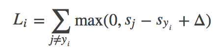
（其中yi是样本i的真实标签，sj是该样本在类别j上的线性得分值，三角形是一个常数，表示保护值）

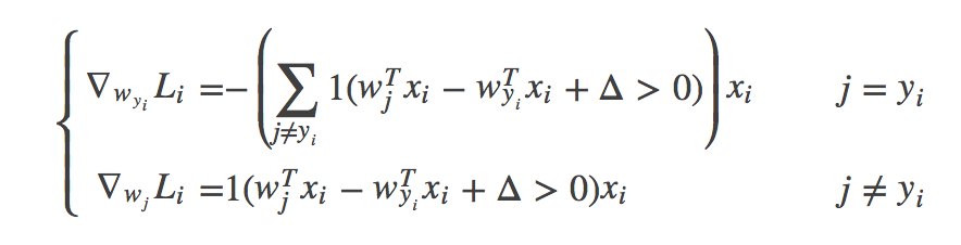
梯度（学会推导）：

（2）两种实现SVM损失和解析梯度的方式

朴素法（两重循环）：

def svm_loss_naive(W, X, y, reg):
  """
  Structured SVM loss function, naive implementation (with loops).

  Inputs have dimension D, there are C classes, and we operate on minibatches
  of N examples.

  Inputs:
  - W: A numpy array of shape (D, C) containing weights.
  - X: A numpy array of shape (N, D) containing a minibatch of data.
  - y: A numpy array of shape (N,) containing training labels; y[i] = c means
    that X[i] has label c, where 0 <= c < C.
  - reg: (float) regularization strength

  Returns a tuple of:
  - loss as single float
  - gradient with respect to weights W; an array of same shape as W
  """
  dW = np.zeros(W.shape) # initialize the gradient as zero

  # compute the loss and the gradient
  num_classes = W.shape[1]
  num_train = X.shape[0]
  loss = 0.0
  for i in xrange(num_train):
    scores = X[i].dot(W)
    correct_class_score = scores[y[i]]
    for j in xrange(num_classes):
      if j == y[i]:
        continue
      margin = scores[j] - correct_class_score + 1 # note delta = 1
      if margin > 0:
        dW[:, j] += X[i, :]
        dW[:, y[i]] += -X[i, :]
        loss += margin

  # Right now the loss is a sum over all training examples, but we want it
  # to be an average instead so we divide by num_train.
  loss /= num_train
  dW /= num_train

  # Add regularization to the loss.
  loss += reg * np.sum(W * W)
  dW += 2 * reg * W
  #############################################################################
  # TODO:                                                                     #
  # Compute the gradient of the loss function and store it dW.                #
  # Rather that first computing the loss and then computing the derivative,   #
  # it may be simpler to compute the derivative at the same time that the     #
  # loss is being computed. As a result you may need to modify some of the    #
  # code above to compute the gradient.                                       #
  #############################################################################

  return loss, dW

完全向量法：
很有技巧性，使用数组的广播来计算loss。由于观察到每次的梯度是训练集向量的线性叠加，使用计算loss中产生的中间矩阵lossMat来构造该线性权重矩阵H，该权重矩阵H大小为n*10，对于Hij，当样本i的正确分类不为j，如果max（si-syi+1）>0，则Hij为1，否则为0；当样本i的正确分类为j，则Hij为10个分类中max（si-syi+1）大于0的个数的倒数。其中max（si-syi+1）就是lossMat矩阵中的值。

def svm_loss_vectorized(W, X, y, reg):
  """
  Structured SVM loss function, vectorized implementation.

  Inputs and outputs are the same as svm_loss_naive.
  """
  loss = 0.0
  dW = np.zeros(W.shape) # initialize the gradient as zero
  num_classes = W.shape[1]
  num_train = X.shape[0]
  #############################################################################
  # TODO:                                                                     #
  # Implement a vectorized version of the structured SVM loss, storing the    #
  # result in loss.                                                           #
  #############################################################################
  scores = X.dot(W)
  rightClassScores = scores[range(0, num_train), list(y)].reshape(num_train, 1)
  lossMat = scores - rightClassScores + 1
  
  lossMat[lossMat < 0] = 0.0
  loss = (np.sum(lossMat) - num_train) / num_train
  
  #############################################################################
  #                             END OF YOUR CODE                              #
  #############################################################################
  

  #############################################################################
  # TODO:                                                                     #
  # Implement a vectorized version of the gradient for the structured SVM     #
  # loss, storing the result in dW.                                           #
  #                                                                           #
  # Hint: Instead of computing the gradient from scratch, it may be easier    #
  # to reuse some of the intermediate values that you used to compute the     #
  # loss.                                                                     #
  #############################################################################
  lossMat[lossMat > 0] = 1.0
  lossMat[range(0, num_train), list(y)] = -np.sum(lossMat, axis=1) + 1
  dW = X.T.dot(lossMat) / num_train + 2 * reg * W
  #############################################################################
  #                             END OF YOUR CODE                              #
  #############################################################################

  return loss, dW

实验表明完全向量化的代码比朴素法快十几倍。

（3）完整代码

- 实现了SVM完全向量化的损失函数
- 实现了解析梯度完全向量化的表达式
- 使用数值梯度检查了解析梯度的正确性
- 使用验证集调参：学习速率和正则化强度
- 实现了优化损失函数的SGD算法
- 可视化最终学习权重，可以看出线性分类器相当于为每个类学出一个模版（对应权重矩阵的一行），进行模版匹配(可视化的方法是将权重进行归一化，然后乘以255)。

 https://nbviewer.jupyter.org/github/coldyan123/Assignments1/blob/master/svm.ipynb

 

 3 softmax

（1）损失函数及梯度

样本i的损失函数：

梯度：

 

(2) 两种实现softmax损失及其梯度的方式

朴素法：

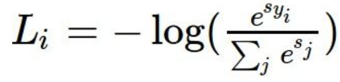
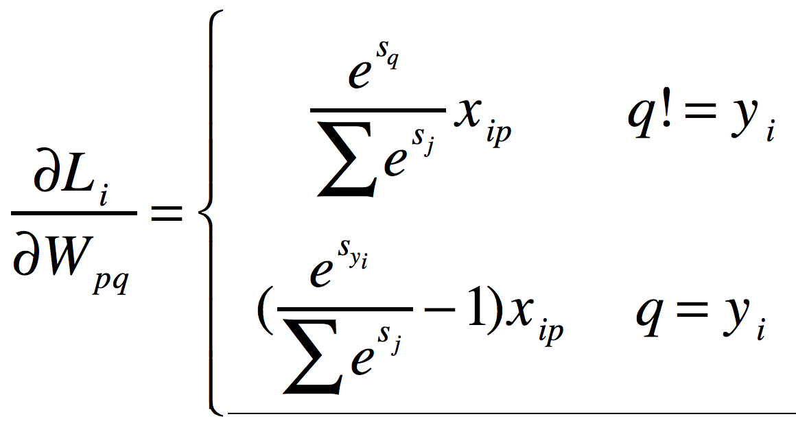
def softmax_loss_naive(W, X, y, reg):
  """
  Softmax loss function, naive implementation (with loops)

  Inputs have dimension D, there are C classes, and we operate on minibatches
  of N examples.

  Inputs:
  - W: A numpy array of shape (D, C) containing weights.
  - X: A numpy array of shape (N, D) containing a minibatch of data.
  - y: A numpy array of shape (N,) containing training labels; y[i] = c means
    that X[i] has label c, where 0 <= c < C.
  - reg: (float) regularization strength

  Returns a tuple of:
  - loss as single float
  - gradient with respect to weights W; an array of same shape as W
  """
  # Initialize the loss and gradient to zero.
  loss = 0.0
  dW = np.zeros_like(W)

  #############################################################################
  # TODO: Compute the softmax loss and its gradient using explicit loops.     #
  # Store the loss in loss and the gradient in dW. If you are not careful     #
  # here, it is easy to run into numeric instability. Don't forget the        #
  # regularization!                                                           #
  #############################################################################
  train_num = X.shape[0]
  dim = X.shape[1]
  class_num = W.shape[1]
  for i in range(0, train_num):
      scores = X[i].dot(W)
      Sum = 0
      for j in range(0, class_num):
          Sum += math.exp(scores[j])
      for j in range(0, class_num):
          if j == y[i]:
              dW[:, j] += (math.exp(scores[y[i]]) / Sum - 1) * X[i]
          else:
              dW[:, j] += math.exp(scores[j]) / Sum * X[i]
      loss += -math.log(math.exp(scores[y[i]]) / Sum)    
  loss /= train_num
  dW /= train_num
  dW += 2 * reg * W
  
    
  #############################################################################
  #                          END OF YOUR CODE                                 #
  #############################################################################

  return loss, dW

完全向量法：

这里与SVM的完全向量实现思路基本相同，都是构造出样本对于梯度的权重贡献矩阵H。搞懂了SVM的再来写这个简直易如反掌。

def softmax_loss_vectorized(W, X, y, reg):
  """
  Softmax loss function, vectorized version.

  Inputs and outputs are the same as softmax_loss_naive.
  """
  # Initialize the loss and gradient to zero.
  loss = 0.0
  dW = np.zeros_like(W)

  #############################################################################
  # TODO: Compute the softmax loss and its gradient using no explicit loops.  #
  # Store the loss in loss and the gradient in dW. If you are not careful     #
  # here, it is easy to run into numeric instability. Don't forget the        #
  # regularization!                                                           #
  #############################################################################
  train_num = X.shape[0]
  dim = X.shape[1]
  class_num = W.shape[1]
  
  scores = X.dot(W)
  exp_scores = np.exp(scores)
  tmp = exp_scores[range(0, train_num), y] / np.sum(exp_scores, axis=1)
  loss = np.sum(-np.log(tmp)) / train_num
  
  H = exp_scores / np.sum(exp_scores, axis=1).reshape((train_num, 1))
  H[range(0, train_num), y] -= 1
  dW = X.T.dot(H) / train_num + 2 * reg * W 
  #############################################################################
  #                          END OF YOUR CODE                                 #
  #############################################################################

  return loss, dW

（3）完整代码

- 实现了Softmax分类器完全向量化的损失函数

- 实现了解析梯度完全向量化的代码
- 用数值梯度检查了实现
- 使用验证集调整学习速度和正则化强度
- 使用SGD优化损失函数
- 可视化最终学习权重

 https://nbviewer.jupyter.org/github/coldyan123/Assignments1/blob/master/softmax.ipynb

4 两层神经网络

（1）softMax loss和梯度的计算（完全向量法）

loss的计算非常简单：

# Compute the loss
    loss = None
    #############################################################################
    # TODO: Finish the forward pass, and compute the loss. This should include  #
    # both the data loss and L2 regularization for W1 and W2. Store the result  #
    # in the variable loss, which should be a scalar. Use the Softmax           #
    # classifier loss.                                                          #
    #############################################################################
    exp_scores = np.exp(scores)
    loss = np.sum(-np.log(exp_scores[range(0, N), y] / np.sum(exp_scores, axis=1)))
    loss /= N
    loss += reg * (np.sum(W1 * W1) + np.sum(W2 * W2))
    #############################################################################
    #                              END OF YOUR CODE                             #
    ############################################################################

梯度的计算比较复杂，主要难在涉及到了矩阵对矩阵的导数（WX+B对W或X的导数），以及Relu层的导数。

a 矩阵线性变换的导数是一个常用的结论，需要记住（使用平铺矩阵jocabian法可以推出这个结论）：

（等式右边是左乘右乘还是转置不用记忆，根据维度相容的方法可以现推出来）

b ReLu层的导数

Relu层表示为：

其中是对矩阵A进行逐元素地max（0，Aij）操作的，所以很容易得出：

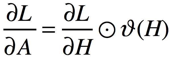
其中，运算符表示逐元素想乘，函数表示将矩阵H中的元素大于0的置为1，其余置为0。

因此梯度的计算代码如下：

# Backward pass: compute gradients
    grads = {}
    #############################################################################
    # TODO: Compute the backward pass, computing the derivatives of the weights #
    # and biases. Store the results in the grads dictionary. For example,       #
    # grads['W1'] should store the gradient on W1, and be a matrix of same size #
    #############################################################################
    #cal gradsOfLossByScore
    gradsOfLossByScore = exp_scores / np.sum(exp_scores, axis=1).reshape((N,1))
    gradsOfLossByScore[range(0, N), y] -= 1
    #cal grads['b2'] 
    gradsOfLossByb2 = gradsOfLossByScore
    grads['b2'] = np.sum(gradsOfLossByb2, axis=0) / N
    #
    grads['W2'] = h.T.dot(gradsOfLossByScore) / N + 2 * reg * W2
    #
    gradsOfLossByh = gradsOfLossByScore.dot(W2.T)
    gradsOfLossBya1 = gradsOfLossByh * (h > 0)
    gradsOfLossByb1 = gradsOfLossBya1
    grads['b1'] = np.sum(gradsOfLossByb1, axis=0) / N
    grads['W1'] = X.T.dot(gradsOfLossBya1) / N + 2 * reg * W1 
    #############################################################################
    #                              END OF YOUR CODE                             #
    #############################################################################

（2）完整代码

 在这项练习中，我使用了高效的向量化代码实现了两层全连接神经网络的前向传播，反向传播，训练以及预测。并通过调节超参数，在验证集上达到了0.525的准确率，测试集上达到了0.519的准确率。

https://nbviewer.jupyter.org/github/coldyan123/Assignments1/blob/master/two_layer_net.ipynb 

（3）关于反向传播的心得体会

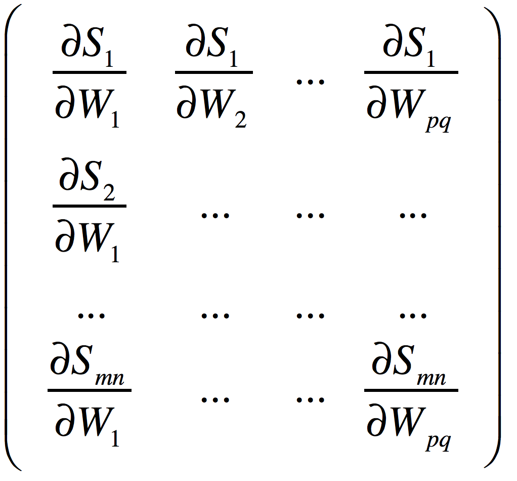
　　在反向传播中，我们使用上游传过来的梯度乘以jocabian矩阵，得到特定参数的梯度，或者是使梯度往下传。但是注意，jocobian矩阵的定义是向量对向量的导数结果，如果遇到向量对矩阵，或者矩阵对矩阵的时候，我们应该用什么来乘以上游梯度呢？考察下面一个例子：

       问题：已知上游传过来的梯度（或称为G），并且有，要求梯度。其中。

　　解法：在这个例子中，我们仍然使用雅可比矩阵进行传播，但是首先需要将S矩阵平展成一个（1，mn）的向量，将W矩阵平展成一个（1，pq）的向量，得到的雅可比矩阵是（mn，pq）大小的。然后我们将上游梯度平展成（1，mn）的向量，使用这个向量乘以雅可比矩阵，得到（1，pq）的向量，将这个向量恢复成（p，q）的形状，就是我们要求的梯度矩阵。

      证明：现在证明上面解法的正确性。

　　记分别为三个矩阵平展开之后的第i个元素，那么，得到的（mn，pq）的雅可比矩阵如下：

           

      而G展开后为。将其乘以雅可比矩阵，得到向量：。

      这个向量中的第k个元素为：

　　 

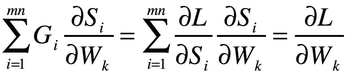
      很明显，将其恢复成（p，q）的形状就是要求的梯度矩阵。

 5 图像特征实验

　　这一部分验证了提取一些图像特征能够达到更高的分类准确率。提取的特征有HOG和color histogram，用到已经实现的SVM和两层神经网络上。经过调参，神经网络在验证集上准确率超过了60%，测试集上达到了58.3%。

    完整代码：

https://nbviewer.jupyter.org/github/coldyan123/Assignments1/blob/master/features.ipynb