import numpy as np
import matplotlib as mpl
import matplotlib.pyplot as plt

import random
#sigmoid函数定义
def sigmoid(x):
# print('sigmoid:',x,1.0 / (1+math.exp(-x)))
return 1.0 / (1+ np.exp(-x))
#模拟数据
x = [-2,6,-2,7,-3,3,0,8,1,10,2,12,2,5,3,6,4,5,2,15,1,10,4,7,4,11,0,3,-1,4,1,5,3,11,4,5]
x = x * 100
#转换成两列的矩阵
x = np.array(x).reshape(-1,2)
# print('x:',x,len(x))
x1 = x[:,0]
x2 = x[:,1]
# print(x1,len(x1))
# print(x2)
y = [1,1,0,1,1,1,0,0,0,1,1,0,1,0,0,0,1,1]
y = y * 100
y = np.array(y).reshape(-1,1)
y1 = y[:,0]
print('len(y):',len(y))
# a = 0.1 #学习步长 alpha
o0 = 1 #线性参数
o1 = 1
o2 = 1
O0=[]
O1=[]
O2=[]
q=[]
result = []
#随机梯度下降求参
dataindex = list(range(len(y)))
for i in range(len(y)):
a = 6/(i+1) +0.01
num = random.randint(0, len(dataindex) - 1)
index = dataindex[num]
# print('index:',index)
# print(x[i],x[i][0])
w = o0 + o1 * x[index][0] +o2 * x[index][1]
# print('w:',w)
h = sigmoid(w)
error = y[index] - h
q.append(error)
# print(num,len(num_list))
del (dataindex[num])
# print(h,y[i])
o0 = o0 + a * error * 1 #梯度上升求最大似然估计的参数值
o1 = o1 + a * error * x[index][0]
o2 = o2 + a * error * x[index][1]
O0.append(o0)
O1.append(o1)
O2.append(o2)
print(o0,o1,o2)
#测试参数
test_x = [-2,6,-2,7,-3,3,0,8,1,10,2,12,2,5,3,6,4,5,2,15,1,10,4,7,4,11,0,3,-1,4,1,5,3,11,4,5]
test_y = [1,1,0,1,1,1,0,0,0,1,1,0,1,0,0,0,1,1]
yescount = 0
for i in range(len(test_y)):
test_w = o0 + o1 * x[i][0] +o2 * x[i][1]
test_h = sigmoid(test_w)
print('测试:',test_w,y[i])
if test_h < 0.5:
result = 0
else:
result = 1
if result == y[i]:
yescount += 1
# print('正确')
print('总共{}个,正确了{}个,正确率为:{}'.format(len(test_y),yescount,yescount/len(test_y)))
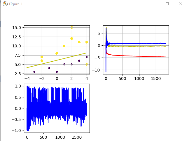
#参数求好了画图
fig = plt.figure()
#第一幅数据散点和回归分割线
line_x = np.arange(-4,4,0.1) #横坐标
line_y = (-o0-o1*line_x) / o2 #分割线
ax2 = fig.add_subplot(221)
ax2.scatter(x1,x2,10*(y1+1),10*(y1+1)) #测试数据的散点图
plt.grid()
plt.plot(line_x,line_y,'y-')
#第二幅参数o1 o2 o3 的变化图
ax3 = fig.add_subplot(222)
plt.grid()
plt.plot(range(len(y)),O0,'r-')
plt.plot(range(len(y)),O1,'y-')
plt.plot(range(len(y)),O2,'b-')
#第三幅数据误差error图
ax4 = fig.add_subplot(223)
plt.plot(range(len(y)),q,'b-')
plt.show()