The source code of this demo project:
https://github.com/xiaoweige/ImageSearch
Here’s a quick overview:
- What we’re going to do: Build an image search engine, from start to finish, using The Hobbit and Lord of the Rings screenshots.
- What you’ll learn: The 4 steps required to build an image search engine, with code examples included. From these examples, you’ll be able to build image search engines of your own.
- What you need: Python, NumPy, and OpenCV. A little knowledge of basic image concepts, such as pixels and histograms, would help, but is absolutely not required. This blog post is meant to be a How-To, hands on guide to building an image search engine.
OpenCV and Python versions:
This example will run on Python 2.7 and OpenCV 2.4.X.
But before I dive into the details of building an image search engine, let’s check out our dataset of The Hobbit and Lord of the Rings screenshots:
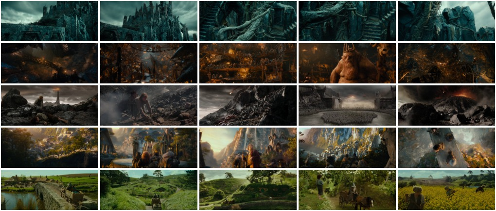
Figure 1: Our dataset of The Hobbit and Lord of the Rings screenshots. We have 25 total images of 5 different categories including Dol Guldur, the Goblin Town, Mordor/The Black Gate, Rivendell, and The Shire.
So as you can see, we have a total of 25 different images in our dataset, five per category. Our categories include:
- Dol Guldur: “The dungeons of the Necromancer”, Sauron’s stronghold in Mirkwood.
- Goblin Town: An Orc town in the Misty Mountains, home of The Goblin King.
- Mordor/The Black Gate: Sauron’s fortress, surrounded by mountain ranges and volcanic plains.
- Rivendell: The Elven outpost in Middle-earth.
- The Shire: Homeland of the Hobbits.
The images from Dol Guldur, the Goblin Town, and Rivendell are from The Hobbit: An Unexpected Journey. Our Shire images are from The Lord of the Rings: The Fellowship of the Ring. And finally, our Mordor/Black Gate screenshots from The Lord of the Rings: The Return of the King.
The Goal:
The first thing we are going to do is index the 25 images in our dataset. Indexing is the process of quantifying our dataset by using an image descriptor to extract features from each image and storing the resulting features for later use, such as performing a search.
An image descriptor defines how we are quantifying an image, hence extracting features from an image is called describing an image. The output of an image descriptor is a feature vector, an abstraction of the image itself. Simply put, it is a list of numbers used to represent an image.
Two feature vectors can be compared using a distance metric. A distance metric is used to determine how “similar” two images are by examining the distance between the two feature vectors. In the case of an image search engine, we give our script a query image and ask it to rank the images in our index based on how relevant they are to our query.
Think about it this way. When you go to Google and type “Lord of the Rings” into the search box, you expect Google to return pages to you that are relevant to Tolkien’s books and the movie franchise. Similarly, if we present an image search engine with a query image, we expect it to return images that are relevant to the content of image — hence, we sometimes call image search engines by what they are more commonly known in academic circles as Content Based Image Retrieval (CBIR) systems.
So what’s the overall goal of our Lord of the Rings image search engine?
The goal, given a query image from one of our five different categories, is to return the category’s corresponding images in the top 10 results.
That was a mouthful. Let’s use an example to make it more clear.
If I submitted a query image of The Shire to our system, I would expect it to give me all 5 Shire images in our dataset back in the first 10 results. And again, if I submitted a query image of Rivendell, I would expect our system to give me all 5 Rivendell images in the first 10 results.
Make sense? Good. Let’s talk about the four steps to building our image search engine.
The 4 Steps to Building an Image Search Engine
On the most basic level, there are four steps to building an image search engine:
- Define your descriptor: What type of descriptor are you going to use? Are you describing color? Texture? Shape?
- Index your dataset: Apply your descriptor to each image in your dataset, extracting a set of features.
- Define your similarity metric: How are you going to define how “similar” two images are? You’ll likely be using some sort of distance metric. Common choices include Euclidean, Cityblock (Manhattan), Cosine, and chi-squared to name a few.
- Searching: To perform a search, apply your descriptor to your query image, and then ask your distance metric to rank how similar your images are in your index to your query images. Sort your results via similarity and then examine them.
Step #1: The Descriptor – A 3D RGB Color Histogram
Our image descriptor is a 3D color histogram in the RGB color space with 8 bins per red, green, and blue channel.
The best way to explain a 3D histogram is to use the conjunctive AND. This image descriptor will ask a given image how many pixels have a Red value that falls into bin #1 AND a Green value that falls into bin #2 AND how many Blue pixels falls into bin #1. This process will be repeated for each combination of bins; however, it will be done in a computationally efficient manner.
When computing a 3D histogram with 8 bins, OpenCV will store the feature vector as an (8, 8, 8) array. We’ll simply flatten it and reshape it to (512,). Once it’s flattened, we can easily compare feature vectors together for similarity.
Ready to see some code? Okay, here we go:
 1 # import the necessary packages
 2 import numpy as np
 3 import cv2
 4
 5 class RGBHistogram:
 6     def __init__(self, bins):
 7         # store the number of bins the histogram will use
 8         self.bins = bins
 9
10     def describe(self, image):
11         # compute a 3D histogram in the RGB colorspace,
12         # then normalize the histogram so that images
13         # with the same content, but either scaled larger
14         # or smaller will have (roughly) the same histogram
15         hist = cv2.calcHist([image], [0, 1, 2],
16             None, self.bins, [0, 256, 0, 256, 0, 256])
17         hist = cv2.normalize(hist)
18
19         # return out 3D histogram as a flattened array
20         return hist.flatten()
As you can see, I have defined a RGBHistogram class. I tend to like to define my image descriptors as classes rather than functions. The reason for this is because you rarely ever extract features from a single image alone. You instead extract features from an entire dataset of images. Furthermore, you expect that the features extracted from all images utilize the same parameters — in this case, the number of bins for the histogram. It wouldn’t make much sense to extract a histogram using 32 bins from one image and then 128 bins for another image if you intend on comparing them for similarity.
Let’s take the code apart and understand what’s going on:
- Lines 6-8: Here I am defining the constructor for the
RGBHistogram. The only parameter we need is the number of bins for each channel in the histogram. Again, this is why I prefer using classes instead of functions for image descriptors — by putting the relevant parameters in the constructor, you ensure that the same parameters are utilized for each image. - Line 10: You guessed it. The describe method is used to “describe” the image and return a feature vector.
- Line 15: Here we extract the actual 3D RGB Histogram (or actually, BGR since OpenCV stores the image as a NumPy array, but with the channels in reverse order). We assume
self.binsis a list of three integers, designating the number of bins for each channel. - Line 16: It’s important that we normalize the histogram in terms of pixel counts. If we used the raw (integer) pixel counts of an image, then shrunk it by 50% and described it again, we would have two different feature vectors for identical images. In most cases, you want to avoid this scenario. We obtain scale invariance by converting the raw integer pixel counts into real-valued percentages. For example, instead of saying bin #1 has 120 pixels in it, we would say bin #1 has 20% of all pixels in it. Again, by using the percentages of pixel counts rather than raw, integer pixel counts, we can assure that two identical images, differing only in size, will have (roughly) identical feature vectors.
- Line 20: When computing a 3D histogram, the histogram will be represented as a NumPy array with
(N, N, N)bins. In order to more easily compute the distance between histograms, we simply flatten this histogram to have a shape of(N ** 3,). Example:When we instantiate our RGBHistogram, we will use 8 bins per channel. Without flattening our histogram, the shape would be(8, 8, 8). But by flattening it, the shape becomes(512,).
Now that we have defined our image descriptor, we can move on to the process of indexing our dataset.
Step #2: Indexing our Dataset
Okay, so we’ve decided that our image descriptor is a 3D RGB histogram. The next step is to apply our image descriptor to each image in the dataset.
This simply means that we are going to loop over our 25 image dataset, extract a 3D RGB histogram from each image, store the features in a dictionary, and write the dictionary to file.
Yep, that’s it.
In reality, you can make indexing as simple or complex as you want. Indexing is a task that is easily made parallel. If we had a four core machine, we could divide the work up between the four cores and speedup the indexing process. But since we only have 25 images, that’s pretty silly, especially given how fast it is to compute a histogram.
Let’s dive into some code:
 1 # import the necessary packages
 2 from pyimagesearch.rgbhistogram import RGBHistogram
 3 import argparse
 4 import cPickle
 5 import glob
 6 import cv2
 7
 8 # construct the argument parser and parse the arguments
 9 ap = argparse.ArgumentParser()
10 ap.add_argument("-d", "--dataset", required = True,
11     help = "Path to the directory that contains the images to be indexed")
12 ap.add_argument("-i", "--index", required = True,
13     help = "Path to where the computed index will be stored")
14 args = vars(ap.parse_args())
15
16 # initialize the index dictionary to store our our quantifed
17 # images, with the 'key' of the dictionary being the image
18 # filename and the 'value' our computed features
19 index = {}
Alright, the first thing we are going to do is import the packages we need. I’ve decided to store the RGBHistogram class in a module called pyimagesearch. I mean, it only makes sense, right? We’ll use cPickle to dump our index to disk. And we’ll use glob to get the paths of the images we are going to index.
The --dataset argument is the path to where our images are stored on disk and the --indexoption is the path to where we will store our index once it has been computed.
Finally, we’ll initialize our index — a builtin Python dictionary type. The key for the dictionary will be the image filename. We’ve made the assumption that all filenames are unique, and in fact, for this dataset, they are. The value for the dictionary will be the computed histogram for the image.
Using a dictionary for this example makes the most sense, especially for explanation purposes. Given a key, the dictionary points to some other object. When we use an image filename as a key and the histogram as the value, we are implying that a given histogram H is used to quantify and represent the image with filename K.
Again, you can make this process as simple or as complicated as you want. More complex image descriptors make use of term frequency-inverse document frequency weighting (tf-idf) and an inverted index, but we are going to stay clear of that for now. Don’t worry though, I’ll have plenty of blog posts discussing how we can leverage more complicated techniques, but for the time being, let’s keep it simple.
1 # initialize our image descriptor -- a 3D RGB histogram with
2 # 8 bins per channel
3 desc = RGBHistogram([8, 8, 8])
Here we instantiate our RGBHistogram. Again, we will be using 8 bins for each, red, green, and blue channel, respectively.
 1 # use glob to grab the image paths and loop over them
 2 for imagePath in glob.glob(args["dataset"] + "/*.jpg"):
 3     # extract our unique image ID (i.e. the filename)
 4     ###*** the original line below doesn't work in windows, the best fix is to
 5     #  use a generic solution using os.path pnd@oct2015
 6     #k = imagePath[imagePath.rfind("/") + 1:]
 7         j, k = os.path.split(imagePath)
 8
 9
10     # load the image, describe it using our RGB histogram
11     # descriptor, and update the index
12     image = cv2.imread(imagePath)
13     features = desc.describe(image)
14     index[k] = features
Here is where the actual indexing takes place. Let’s break it down:
- Line 2: We use
globto grab the image paths and start to loop over our dataset. - Line 4: We extract the “key” for our dictionary. All filenames are unique in this sample dataset, so the filename itself will be enough to serve as the key.
- Line 8-10: The image is loaded off disk and we then use our
RGBHistogramto extract a histogram from the image. The histogram is then stored in the index.
1 # we are now done indexing our image -- now we can write our
2 # index to disk
3 f = open(args["index"], "w")
4 f.write(cPickle.dumps(index))
5 f.close()
Now that our index has been computed, let’s write it to disk so we can use it for searching later on.
Step #3: The Search
We now have our index sitting on disk, ready to be searched.
The problem is, we need some code to perform the actual search. How are we going to compare two feature vectors and how are we going to determine how similar they are?
This question is better addressed first with some code, then I’ll break it down.
 1 # import the necessary packages
 2 import numpy as np
 3
 4 class Searcher:
 5     def __init__(self, index):
 6         # store our index of images
 7         self.index = index
 8
 9     def search(self, queryFeatures):
10         # initialize our dictionary of results
11         results = {}
12
13         # loop over the index
14         for (k, features) in self.index.items():
15             # compute the chi-squared distance between the features
16             # in our index and our query features -- using the
17             # chi-squared distance which is normally used in the
18             # computer vision field to compare histograms
19             d = self.chi2_distance(features, queryFeatures)
20
21             # now that we have the distance between the two feature
22             # vectors, we can udpate the results dictionary -- the
23             # key is the current image ID in the index and the
24             # value is the distance we just computed, representing
25             # how 'similar' the image in the index is to our query
26             results[k] = d
27
28         # sort our results, so that the smaller distances (i.e. the
29         # more relevant images are at the front of the list)
30         results = sorted([(v, k) for (k, v) in results.items()])
31
32         # return our results
33         return results
34
35     def chi2_distance(self, histA, histB, eps = 1e-10):
36         # compute the chi-squared distance
37         d = 0.5 * np.sum([((a - b) ** 2) / (a + b + eps)
38             for (a, b) in zip(histA, histB)])
39
40         # return the chi-squared distance
41         return d
First off, most of this code is just comments. Don’t be scared that it’s 41 lines. If you haven’t already guessed, I like well-commented code. Let’s investigate what’s going on:
- Lines 4-7: The first thing I do is define a
Searcherclass and a constructor with a single parameter — theindex. Thisindexis assumed to be the index dictionary that we wrote to file during the indexing step. - Line 11: We define a dictionary to store our
results. The key is the image filename (from the index) and the value is how similar the given image is to the query image. - Lines 14-26: Here is the part where the actual searching takes place. We loop over the image filenames and corresponding features in our index. We then use the chi-squared distance to compare our color histograms. The computed distance is then stored in the
resultsdictionary, indicating how similar the two images are to each other. - Lines 30-33: The results are sorted in terms of relevancy (the smaller the chi-squared distance, the relevant/similar) and returned.
- Lines 35-41: Here we define the chi-squared distance function used to compare the two histograms. In general, the difference between large bins vs. small bins is less important and should be weighted as such. This is exactly what the chi-squared distance does. We provide an
epsilondummy value to avoid those pesky “divide by zero” errors. Images will be considered identical if their feature vectors have a chi-squared distance of zero. The larger the distance gets, the less similar they are.
So there you have it, a Python class that can take an index and perform a search. Now it’s time to put this searcher to work.
Note: For those who are more academically inclined, you might want to check out The Quadratic-Chi Histogram Distance Family from the ECCV ’10 conference if you are interested in histogram distance metrics.
Step #4: Performing a Search
Finally. We are closing in on a functioning image search engine.
But we’re not quite there yet. We need a little extra code to handle loading the images off disk and performing the search:
 1 # import the necessary packages
 2 from pyimagesearch.searcher import Searcher
 3 import numpy as np
 4 import argparse
 5 import cPickle
 6 import cv2
 7
 8 # construct the argument parser and parse the arguments
 9 ap = argparse.ArgumentParser()
10 ap.add_argument("-d", "--dataset", required = True,
11     help = "Path to the directory that contains the images we just indexed")
12 ap.add_argument("-i", "--index", required = True,
13     help = "Path to where we stored our index")
14 args = vars(ap.parse_args())
15
16 # load the index and initialize our searcher
17 index = cPickle.loads(open(args["index"]).read())
18 searcher = Searcher(index)
First things first. Import the packages that we will need. As you can see, I’ve stored our Searcher class in the pyimagesearch module. We then define our arguments in the same manner that we did during the indexing step. Finally, we use cPickle to load our index off disk and initialize our Searcher.
 1 # loop over images in the index -- we will use each one as
 2 # a query image
 3 for (query, queryFeatures) in index.items():
 4     # perform the search using the current query
 5     results = searcher.search(queryFeatures)
 6
 7     # load the query image and display it
 8     path = args["dataset"] + "/%s" % (query)
 9     queryImage = cv2.imread(path)
10     cv2.imshow("Query", queryImage)
11     print "query: %s" % (query)
12
13     # initialize the two montages to display our results --
14     # we have a total of 25 images in the index, but let's only
15     # display the top 10 results; 5 images per montage, with
16     # images that are 400x166 pixels
17     montageA = np.zeros((166 * 5, 400, 3), dtype = "uint8")
18     montageB = np.zeros((166 * 5, 400, 3), dtype = "uint8")
19
20     # loop over the top ten results
21     for j in xrange(0, 10):
22         # grab the result (we are using row-major order) and
23         # load the result image
24         (score, imageName) = results[j]
25         path = args["dataset"] + "/%s" % (imageName)
26         result = cv2.imread(path)
27         print "	%d. %s : %.3f" % (j + 1, imageName, score)
28
29         # check to see if the first montage should be used
30         if j < 5:
31             montageA[j * 166:(j + 1) * 166, :] = result
32
33         # otherwise, the second montage should be used
34         else:
35             montageB[(j - 5) * 166:((j - 5) + 1) * 166, :] = result
36
37     # show the results
38     cv2.imshow("Results 1-5", montageA)
39     cv2.imshow("Results 6-10", montageB)
40     cv2.waitKey(0)
Most of this code handles displaying the results. The actual “search” is done in a single line (#31). Regardless, let’s examine what’s going on:
- Line 3: We are going to treat each image in our index as a query and see what results we get back. Normally, queries are external and not part of the dataset, but before we get to that, let’s just perform some example searches.
- Line 5: Here is where the actual search takes place. We treat the current image as our query and perform the search.
- Lines 8-11: Load and display our query image.
- Lines 17-35: In order to display the top 10 results, I have decided to use two montage images. The first montage shows results 1-5 and the second montage results 6-10. The name of the image and distance is provided on Line 27.
- Lines 38-40: Finally, we display our search results to the user.
So there you have it. An entire image search engine in Python. Let’s see how this thing performs:
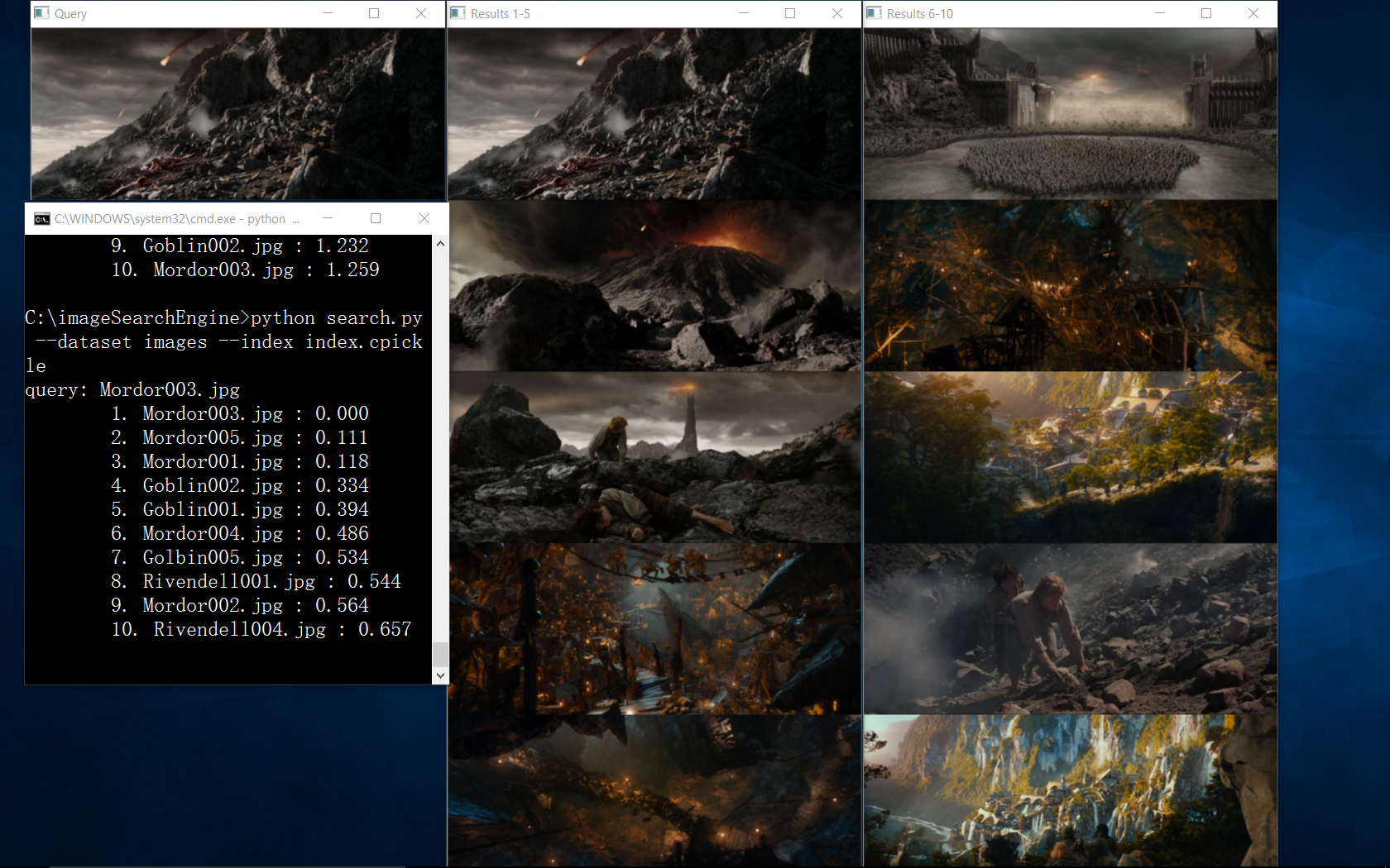
Figure 2: Search Results using Mordor-002.png as a query. Our image search engine is able to return images from Mordor and the Black Gate.
Let’s start at the ending of The Return of the King using Frodo and Sam’s ascent into the volcano as our query image. As you can see, our top 5 results are from the “Mordor” category.
Perhaps you are wondering why the query image of Frodo and Sam is also the image in the #1 result position? Well, let’s think back to our chi-squared distance. We said that an image would be considered “identical” if the distance between the two feature vectors is zero. Since we are using images we have already indexed as queries, they are in fact identical and will have a distance of zero. Since a value of zero indicates perfect similarity, the query image appears in the #1 result position.
Now, let’s try another image, this time using The Goblin King in Goblin Town:

Figure 3: Search Results using Goblin-004.png as a query. The top 5 images returned are from Goblin Town.
Bonus: External Queries
As of right now, I’ve only shown you how to perform a search using images that are already in your index. But clearly, this is not how all image search engines work. Google allows you to upload an image of your own. TinEye allows you to upload an image of your own. Why can’t we? Let’s see how we can perform a search using an image that we haven’t already indexed:
 1 # import the necessary packages
 2 from pyimagesearch.rgbhistogram import RGBHistogram
 3 from pyimagesearch.searcher import Searcher
 4 import numpy as np
 5 import argparse
 6 import cPickle
 7 import cv2
 8
 9 # construct the argument parser and parse the arguments
10 ap = argparse.ArgumentParser()
11 ap.add_argument("-d", "--dataset", required = True,
12     help = "Path to the directory that contains the images we just indexed")
13 ap.add_argument("-i", "--index", required = True,
14     help = "Path to where we stored our index")
15 ap.add_argument("-q", "--query", required = True,
16     help = "Path to query image")
17 args = vars(ap.parse_args())
18
19 # load the query image and show it
20 queryImage = cv2.imread(args["query"])
21 cv2.imshow("Query", queryImage)
22 print "query: %s" % (args["query"])
23
24 # describe the query in the same way that we did in
25 # index.py -- a 3D RGB histogram with 8 bins per
26 # channel
27 desc = RGBHistogram([8, 8, 8])
28 queryFeatures = desc.describe(queryImage)
29
30 # load the index perform the search
31 index = cPickle.loads(open(args["index"]).read())
32 searcher = Searcher(index)
33 results = searcher.search(queryFeatures)
34
35 # initialize the two montages to display our results --
36 # we have a total of 25 images in the index, but let's only
37 # display the top 10 results; 5 images per montage, with
38 # images that are 400x166 pixels
39 montageA = np.zeros((166 * 5, 400, 3), dtype = "uint8")
40 montageB = np.zeros((166 * 5, 400, 3), dtype = "uint8")
41
42 # loop over the top ten results
43 for j in xrange(0, 10):
44     # grab the result (we are using row-major order) and
45     # load the result image
46     (score, imageName) = results[j]
47     path = args["dataset"] + "/%s" % (imageName)
48     result = cv2.imread(path)
49     print "	%d. %s : %.3f" % (j + 1, imageName, score)
50
51     # check to see if the first montage should be used
52     if j < 5:
53         montageA[j * 166:(j + 1) * 166, :] = result
54
55     # otherwise, the second montage should be used
56     else:
57         montageB[(j - 5) * 166:((j - 5) + 1) * 166, :] = result
58
59 # show the results
60 cv2.imshow("Results 1-5", montageA)
61 cv2.imshow("Results 6-10", montageB)
62 cv2.waitKey(0)
- Lines 2-17: This should feel like pretty standard stuff by now. We are importing our packages and setting up our argument parser, although, you should note the new argument –query. This is the path to our query image.
- Lines 20-21: We’re going to load your query image and show it to you, just in case you forgot what your query image is.
- Lines 27-28: Instantiate our
RGBHistogramwith the exact same number of bins as during our indexing step. I put that in bold and italics just to drive home how important it is to use the same parameters. We then extract features from our query image. - Lines 31-33: Load our index off disk using
cPickleand perform the search. - Lines 39-62: Just as in the code above to perform a search, this code just shows us our results.
Before writing this blog post, I went on Google and downloaded two images not present in our index. One of Rivendell and one of The Shire. These two images will be our queries. Check out the results below:
