生成测试数据
绘图首先需要数据。通过生成一堆的向量,转换为矩阵,得到想要的数据。
data <- c(1:6, 6:1, 6:1, 1:6, (6:1)/10, (1:6)/10, (1:6)/10, (6:1)/10, 1:6, 6:1, 6:1, 1:6, 6:1, 1:6, 1:6, 6:1)
[1] 1.0 2.0 3.0 4.0 5.0 6.0 6.0 5.0 4.0 3.0 2.0 1.0 6.0 5.0
[15] 4.0 3.0 2.0 1.0 1.0 2.0 3.0 4.0 5.0 6.0 0.6 0.5 0.4 0.3
[29] 0.2 0.1 0.1 0.2 0.3 0.4 0.5 0.6 0.1 0.2 0.3 0.4 0.5 0.6
[43] 0.6 0.5 0.4 0.3 0.2 0.1 1.0 2.0 3.0 4.0 5.0 6.0 6.0 5.0
[57] 4.0 3.0 2.0 1.0 6.0 5.0 4.0 3.0 2.0 1.0 1.0 2.0 3.0 4.0
[71] 5.0 6.0 6.0 5.0 4.0 3.0 2.0 1.0 1.0 2.0 3.0 4.0 5.0 6.0
[85] 1.0 2.0 3.0 4.0 5.0 6.0 6.0 5.0 4.0 3.0 2.0 1.0
注意:运算符的优先级
> 1:3+4
[1] 5 6 7
> 1:(3+4)
[1] 1 2 3 4 5 6 7
Vector转为矩阵 (matrix),再转为数据框 (data.frame)
# ncol 指定列数
# byrow 先按行填充数据
# ?matrix 可查看函数的使用方法
# as.data.frame的as系列是转换用的
data <- as.data.frame(matrix(data, ncol=12, byrow=T))

# 增加列的名字
colnames(data) <- c("Zygote","2_cell","4_cell","8_cell","Morula","ICM","ESC","4 week PGC","7 week PGC","10 week PGC","17 week PGC","OOcyte")
# 增加行的名字
rownames(data) <- paste("Gene", 1:8, sep="_")
# 只显示前6行和前4列
head(data)[,1:4]
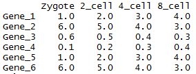
虽然方法比较繁琐,但一个数值矩阵已经获得了。
还有另外2种获取数值矩阵的方式。
- 读入字符串
# 使用字符串的好处是不需要额外提供文件
# 简单测试时可使用,写起来不繁琐,又方便重复
# 尤其适用于在线提问时作为测试案例
> txt <- "ID;Zygote;2_cell;4_cell;8_cell
+ Gene_1;1;2;3;4
+ Gene_2;6;5;4;5
+ Gene_3;0.6;0.5;0.4;0.4"

# 习惯设置quote为空,避免部分基因名字或注释中存在引号,导致读入文件错误。
> data2 <- read.table(text=txt, sep=";", header=T, row.names=1, quote="")
> head(data2)
       Zygote X2_cell X4_cell X8_cell
Gene_1    1.0     2.0     3.0     4.0
Gene_2    6.0     5.0     4.0     5.0
Gene_3    0.6     0.5     0.4     0.4
可以看到列名字中以数字开头的列都加了X。一般要尽量避免行或列名字以数字开头,会给后续分析带去一些困难;另外名字中出现的非字母、数字、下划线、点的字符都会被转为点,也需要注意,尽量只用字母、下划线和数字。
# 读入时,增加一个参数`check.names=F`也可以解决问题。
# 这次数字前没有再加 X 了
> data2 <- read.table(text=txt, sep=";", header=T, row.names=1, quote="", check.names = F)
> head(data2)
       Zygote 2_cell 4_cell 8_cell
Gene_1    1.0    2.0    3.0    4.0
Gene_2    6.0    5.0    4.0    5.0
Gene_3    0.6    0.5    0.4    0.4
- 读入文件
与上一步类似,只是改为文件名,不再赘述。
> data2 <- read.table("filename", sep=";", header=T, row.names=1, quote="")
转换数据格式
数据读入后,还需要一步格式转换。在使用ggplot2作图时,有一种长表格模式是最为常用的,尤其是数据不规则时,更应该使用。
# 如果包没有安装,运行下面一句,安装包
#install.packages(c("reshape2","ggplot2","magrittr"))
library(reshape2)
library(ggplot2)

# 转换前,先增加一列ID列,保存行名字
data$ID <- rownames(data)

# melt:把正常矩阵转换为长表格模式的函数。工作原理是把全部的非id列的数值列转为1列,命名为value;所有字符列转为variable列。
# id.vars 列用于指定哪些列为id列;这些列不会被merge,会保留为完整一列。
data_m <- melt(data, id.vars=c("ID"))
head(data_m)
ID variable value1 Gene_1 Zygote 1.02 Gene_2 Zygote 6.03 Gene_3 Zygote 0.64 Gene_4 Zygote 0.15 Gene_5 Zygote 1.06 Gene_6 Zygote 6.07 Gene_7 Zygote 6.08 Gene_8 Zygote 1.09 Gene_1 2_cell 2.010 Gene_2 2_cell 5.011 Gene_3 2_cell 0.512 Gene_4 2_cell 0.213 Gene_5 2_cell 2.014 Gene_6 2_cell 5.015 Gene_7 2_cell 5.016 Gene_8 2_cell 2.0
分解绘图
数据转换后就可以画图了,分解命令如下:
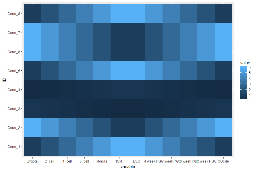
# data_m: 是前面费了九牛二虎之力得到的数据表
# aes: aesthetic的缩写,一般指定整体的X轴、Y轴、颜色、形状、大小等
# 在最开始读入数据时,一般只指定x和y,其它后续指定
p <- ggplot(data_m, aes(x=variable,y=ID))

# 热图就是一堆方块根据其值赋予不同的颜色,所以这里使用fill=value, 用数值做填充色。
p <- p + geom_tile(aes(fill=value))

# ggplot2为图层绘制,一层层添加,存储在p中,在输出p的内容时才会出图。
p

## 如果你没有使用Rstudio或其它R图形版工具,而是在远程登录的服务器上运行的交互式R,需要输入下面的语句,获得输出图形(图形存储于R的工作目录下的Rplots.pdf文件中)
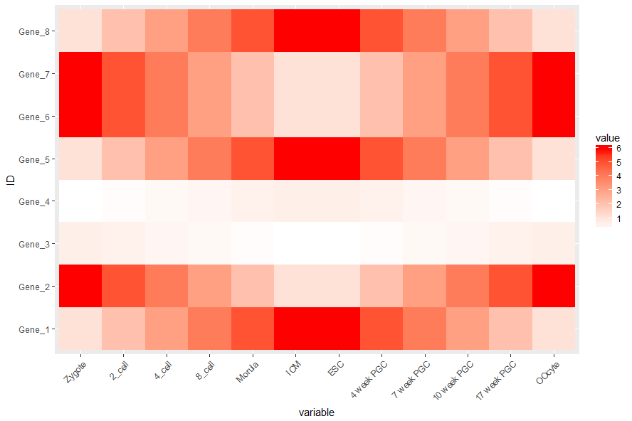
热图出来了,但有点不对劲,横轴重叠一起了。一个办法是调整图像的宽度,另一个是旋转横轴标记
# theme: 是处理图美观的一个函数,可以调整横纵轴label的选择、图例的位置等
# 这里选择X轴标签45度。
# hjust和vjust调整标签的相对位置,具体见
# 简单说,hjust是水平的对齐方式,0为左,1为右,0.5居中,0-1之间可以取任意值。vjust是垂直对齐方式,0底对齐,1为顶对齐,0.5居中,0-1之间可以取任意值
p <- p + theme(axis.text.x=element_text(angle=45, hjust=1, vjust=1))
p
设置想要的颜色
# 连续的数字,指定最小数值代表的颜色和最大数值赋予的颜色
# 注意fill和color的区别,fill是填充,color只针对边缘
p <- p + scale_fill_gradient(low = "white", high = "red")
p
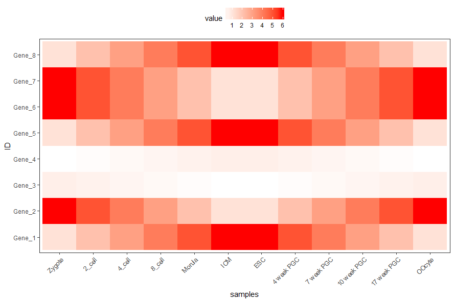
调整legend的位置
# postion可以接受的值有 top, bottom, left, right, 和一个坐标 c(0.05,0.8) (左上角,坐标是相对于图的左下角计算的)
p <- p + theme(legend.position="top")
调整背景和背景格线以及X轴、Y轴的标题(注意灰色的背景没了)
p <- p + xlab("samples") + theme_bw() + theme(panel.grid.major = element_blank()) + theme(legend.key=element_blank())
p
合并以上命令,就得到了下面这个看似复杂的绘图命令
p <- ggplot(data_m, aes(x=variable,y=ID)) + xlab("samples") + theme_bw() + theme(panel.grid.major = element_blank()) + theme(legend.key=element_blank()) + theme(axis.text.x=element_text(angle=45,hjust=1, vjust=1)) + theme(legend.position="top") + geom_tile(aes(fill=value)) + scale_fill_gradient(low = "white", high = "red")
图形存储
图形出来了,就得考虑存储了
# 可以跟输出文件不同的后缀,以获得不同的输出格式
# colormode支持srgb (屏幕)和cmyk (打印,部分杂志需要,看上去有点褪色的感觉)格式
ggsave(p, filename="heatmap.pdf", width=10, height=15, units=c("cm"),colormodel="srgb")
至此,完成了简单的heatmap的绘图。但实际绘制时,经常会碰到由于数值变化很大,导致颜色过于集中,使得图的可读性下降很多。因此需要对数据进行一些处理,具体的下次再说。