zoukankan html css js c++ java

转：SSD详解

原文：http://blog.csdn.net/a8039974/article/details/77592395，

　　http://blog.csdn.net/jesse_mx/article/details/74011886

另外一篇很详细的解析：https://www.cnblogs.com/xuanyuyt/p/7222867.html

SSD github : https://github.com/weiliu89/caffe/tree/ssd

SSD paper : https://arxiv.org/abs/1512.02325

SSD eccv2016 slide pdf : http://download.csdn.NET/download/zy1034092330/9940054

SSD pose estimation paper : http://download.csdn.net/download/zy1034092330/9940059

图1

缩进SSD，全称Single Shot MultiBox Detector，是Wei Liu在ECCV 2016上提出的一种目标检测算法，截至目前是主要的检测框架之一，相比Faster RCNN有明显的速度优势，相比YOLO又有明显的mAP优势（不过已经被CVPR 2017的YOLO9000超越）。SSD具有如下主要特点：

从YOLO中继承了将detection转化为regression的思路，同时一次即可完成网络训练
基于Faster RCNN中的anchor，提出了相似的prior box；
加入基于特征金字塔（Pyramidal Feature Hierarchy）的检测方式，相当于半个FPN思路

本文接下来都以SSD 300为例进行分析。

1 SSD网络结构

图2 SSD网络结构（和代码貌似有点差别）

缩进上图2是原论文中的SSD 300网络结构图。可以看到YOLO在卷积层后接全连接层，即检测时只利用了最高层feature maps（包括Faster RCNN也是如此）；而SSD采用了特征金字塔结构进行检测，即检测时利用了conv4-3，conv-7（FC7），conv6-2，conv7-2，conv8_2，conv9_2这些大小不同的feature maps，在多个feature maps上同时进行softmax分类和位置回归，如图3。

图3 单层feature map预测和特征金字塔预测对比

下面以VGGNet-SSD为例，结合prototxt源文件说一下网络结构。

数据层

这里的数据层类型是AnnotatedData，主要注意下lmdb的source，batch_size以及label_map_file即可。

# 数据层
name: "VGG_VOC0712_SSD_300x300_train"
layer {
  name: "data"
  type: "AnnotatedData"
  top: "data"
  top: "label"
  include {
    phase: TRAIN
  }
  transform_param {
    mirror: true
    mean_value: 104
    mean_value: 117
    mean_value: 123
    resize_param {
      prob: 1
      resize_mode: WARP
      height: 300
       300
      interp_mode: LINEAR
      interp_mode: AREA
      interp_mode: NEAREST
      interp_mode: CUBIC
      interp_mode: LANCZOS4
    }
    emit_constraint {
      emit_type: CENTER
    }
    distort_param {
      brightness_prob: 0.5
      brightness_delta: 32
      contrast_prob: 0.5
      contrast_lower: 0.5
      contrast_upper: 1.5
      hue_prob: 0.5
      hue_delta: 18
      saturation_prob: 0.5
      saturation_lower: 0.5
      saturation_upper: 1.5
      random_order_prob: 0.0
    }
    expand_param {
      prob: 0.5
      max_expand_ratio: 4.0
    }
  }
  data_param {
    source: "examples/VOC0712/VOC0712_trainval_lmdb"
    batch_size: 32
    backend: LMDB
  }
  annotated_data_param {
    batch_sampler {
      max_sample: 1
      max_trials: 1
    }
    batch_sampler {
      sampler {
        min_scale: 0.3
        max_scale: 1.0
        min_aspect_ratio: 0.5
        max_aspect_ratio: 2.0
      }
      sample_constraint {
        min_jaccard_overlap: 0.1
      }
      max_sample: 1
      max_trials: 50
    }
    batch_sampler {
      sampler {
        min_scale: 0.3
        max_scale: 1.0
        min_aspect_ratio: 0.5
        max_aspect_ratio: 2.0
      }
      sample_constraint {
        min_jaccard_overlap: 0.3
      }
      max_sample: 1
      max_trials: 50
    }
    batch_sampler {
      sampler {
        min_scale: 0.3
        max_scale: 1.0
        min_aspect_ratio: 0.5
        max_aspect_ratio: 2.0
      }
      sample_constraint {
        min_jaccard_overlap: 0.5
      }
      max_sample: 1
      max_trials: 50
    }
    batch_sampler {
      sampler {
        min_scale: 0.3
        max_scale: 1.0
        min_aspect_ratio: 0.5
        max_aspect_ratio: 2.0
      }
      sample_constraint {
        min_jaccard_overlap: 0.7
      }
      max_sample: 1
      max_trials: 50
    }
    batch_sampler {
      sampler {
        min_scale: 0.3
        max_scale: 1.0
        min_aspect_ratio: 0.5
        max_aspect_ratio: 2.0
      }
      sample_constraint {
        min_jaccard_overlap: 0.9
      }
      max_sample: 1
      max_trials: 50
    }
    batch_sampler {
      sampler {
        min_scale: 0.3
        max_scale: 1.0
        min_aspect_ratio: 0.5
        max_aspect_ratio: 2.0
      }
      sample_constraint {
        max_jaccard_overlap: 1.0
      }
      max_sample: 1
      max_trials: 50
    }
    label_map_file: "data/VOC0712/labelmap_voc.prototxt"
  }
}

特征提取网络

特征提取网络由两部分构成，VGGNet和新增的8个卷积层，要点有三处。

第一，这个VGGNet不同于原版，是修改过的，全名叫VGG_ILSVRC_16_layers_fc_reduced是作者另一篇论文ParseNet: Looking Wider to See Better的成果，然后被用到了SSD中。

第二，为什么要新增这么8个卷积层？因为在300x300输入下，conv4_3的分辨率为38x38，而到fc7层，也还有19x19，那就必须新增一些卷积层，以产生更多低分辨率的层，方便进行多层特征融合。最终作者选择了6个卷积层作为bottom，分辨率如下图所示，然后依次接上若干检测层。

卷积层	分辨率
conv4_3_norm	38x38
f7	19x19
conv6_2	10x10
conv7_2	5x5
conv8_2	3x3
conv9_2	1x1

第三，只有conv4_3加入了norm，这是为什么呢？原因仍然在论文中ParseNet中，大概是说，因为conv4_3的scale（尺度？）和其它层相比不同，才要加入norm使其均衡一些。

# 特征提取网络
layer {
  name: "conv1_1"
  type: "Convolution"
  bottom: "data"
  top: "conv1_1"
  param {
    lr_mult: 1
    decay_mult: 1
  }
  param {
    lr_mult: 2
    decay_mult: 0
  }
  convolution_param {
    num_output: 64
    pad: 1
    kernel_size: 3
    weight_filler {
      type: "xavier"
    }
    bias_filler {
      type: "constant"
      value: 0
    }
  }
}
#
# 省略很多层
#
layer {
  name: "fc7"
  type: "Convolution"
  bottom: "fc6"
  top: "fc7"
  param {
    lr_mult: 1
    decay_mult: 1
  }
  param {
    lr_mult: 2
    decay_mult: 0
  }
  convolution_param {
    num_output: 1024
    kernel_size: 1
    weight_filler {
      type: "xavier"
    }
    bias_filler {
      type: "constant"
      value: 0
    }
  }
}
layer {
  name: "relu7"
  type: "ReLU"
  bottom: "fc7"
  top: "fc7"
}

# 到此是VGG网络层，从conv1到fc7

layer {
  name: "conv6_1"
  type: "Convolution"
  bottom: "fc7"
  top: "conv6_1"
  param {
    lr_mult: 1
    decay_mult: 1
  }
  param {
    lr_mult: 2
    decay_mult: 0
  }
  convolution_param {
    num_output: 256
    pad: 0
    kernel_size: 1
    stride: 1
    weight_filler {
      type: "xavier"
    }
    bias_filler {
      type: "constant"
      value: 0
    }
  }
}
#
# 省略很多层
#
layer {
  name: "conv9_2_relu"
  type: "ReLU"
  bottom: "conv9_2"
  top: "conv9_2"

# 到此是新增的8层卷积层，从conv6_1到conv9_2

多层融合检测网络

这一部分，作者选择了6个层作为bottom，在其上连接了一系列的检测相关层，这里以f7层为例，看看它作为bottom，连接了那些层。首先是loc相关层，包括fc7_mbox_loc，fc7_mbox_loc_perm和fc7_mbox_loc_flat。

# mbox_loc层，预测box的坐标，其中24=6（default box数量）x4（四个坐标）
layer {
  name: "fc7_mbox_loc"
  type: "Convolution"
  bottom: "fc7"
  top: "fc7_mbox_loc"
  param {
    lr_mult: 1
    decay_mult: 1
  }
  param {
    lr_mult: 2
    decay_mult: 0
  }
  convolution_param {
    num_output: 24
    pad: 1
    kernel_size: 3
    stride: 1
    weight_filler {
      type: "xavier"
    }
    bias_filler {
      type: "constant"
      value: 0
    }
  }
}
# mbox_loc_perm层，将上一层产生的mbox_loc重新排序  
layer {
  name: "fc7_mbox_loc_perm"
  type: "Permute"
  bottom: "fc7_mbox_loc"
  top: "fc7_mbox_loc_perm"
  permute_param {
    order: 0
    order: 2
    order: 3
    order: 1
  }
}
# mbox_loc_flat层，将perm层展平（例如将7x7展成1x49），方便拼接
layer {
  name: "fc7_mbox_loc_flat"
  type: "Flatten"
  bottom: "fc7_mbox_loc_perm"
  top: "fc7_mbox_loc_flat"
  flatten_param {
    axis: 1
  }
}

然后是conf相关层，包括fc7_mbox_conf，fc7_mbox_conf_perm和fc7_mbox_conf_flat。

# mbox_conf层，预测box的类别置信度，126=6（default box数量）x21（总类别数）
layer {
  name: "fc7_mbox_conf"
  type: "Convolution"
  bottom: "fc7"
  top: "fc7_mbox_conf"
  param {
    lr_mult: 1
    decay_mult: 1
  }
  param {
    lr_mult: 2
    decay_mult: 0
  }
  convolution_param {
    num_output: 126
    pad: 1
    kernel_size: 3
    stride: 1
    weight_filler {
      type: "xavier"
    }
    bias_filler {
      type: "constant"
      value: 0
    }
  }
}
# box_conf_perm层，将上一层产生的mbox_conf重新排序 
layer {
  name: "fc7_mbox_conf_perm"
  type: "Permute"
  bottom: "fc7_mbox_conf"
  top: "fc7_mbox_conf_perm"
  permute_param {
    order: 0
    order: 2
    order: 3
    order: 1
  }
}
# mbox_conf_flat层，将perm层展平，方便拼接
layer {
  name: "fc7_mbox_conf_flat"
  type: "Flatten"
  bottom: "fc7_mbox_conf_perm"
  top: "fc7_mbox_conf_flat"
  flatten_param {
    axis: 1
  }
}

最后是priorbox层，就只有fc7_mbox_priorbox

# mbox_priorbox层，根据标注信息，经过转换，在cell中产生box真实值
layer {
  name: "fc7_mbox_priorbox"
  type: "PriorBox"
  bottom: "fc7"
  bottom: "data"
  top: "fc7_mbox_priorbox"
  prior_box_param {
    min_size: 60.0
    max_size: 111.0 # priorbox的上下界为60~111

# first prior: aspect_ratio = 1, box_width = box_height = min_size_; 
# second prior： aspect_ratio = 1， box_width = box_height = sqrt(min_size * max_size);
# others： box_width = min_size_ * sqrt(aspect_ratio); box_height = min_size_ / sqrt(aspect_ratio); 然后对称交换宽高
# 具体详见prior_box_layer.cpp文件

    aspect_ratio: 2
    aspect_ratio: 3 # 共同定义default box数量为6
    flip: true
    clip: false
    variance: 0.1
    variance: 0.1
    variance: 0.2
    variance: 0.2
    step: 16 # 不同层的值不同
    offset: 0.5
  }
}

各个值的计算，详见ssd_pascal.py

mbox_source_layers = ['conv4_3', 'fc7', 'conv6_2', 'conv7_2', 'conv8_2', 'conv9_2']
# in percent %
min_ratio = 20
max_ratio = 90
step = int(math.floor((max_ratio - min_ratio) / (len(mbox_source_layers) - 2)))
min_sizes = []
max_sizes = []
for ratio in xrange(min_ratio, max_ratio + 1, step):
  min_sizes.append(min_dim * ratio / 100.)
  max_sizes.append(min_dim * (ratio + step) / 100.)
min_sizes = [min_dim * 10 / 100.] + min_sizes
max_sizes = [min_dim * 20 / 100.] + max_sizes
steps = [8, 16, 32, 64, 100, 300]
aspect_ratios = [[2], [2, 3], [2, 3], [2, 3], [2], [2]]

下面做一个表格统计一下多层融合检测层的相关重要参数：

bottom层	conv4_3	fc7	conv6_2	conv7_2	conv8_2	conv9_2
分辨率	38x38	19x19	10x10	5x5	3x3	1x1
default box数量	4	6	6	6	4	4
aspect_ratio	2	2,3	2,3	2,3	2	2
steps	8	16	32	64	100	300
loc层num_output	16	24	24	24	16	16
conf层num_output	84	126	126	126	84	84
priorbox层min max size	30~60	60~111	111~162	162~213	213~264	264~315
offset	0.5	0.5	0.5	0.5	0.5	0.5
variance	0.1,0.1,0.2,0.2	0.1,0.1,0.2,0.2	0.1,0.1,0.2,0.2	0.1,0.1,0.2,0.2	0.1,0.1,0.2,0.2	0.1,0.1,0.2,0.2

具体到每一个feature map上获得prior box时，会从这6种中进行选择。如下表和图所示最后会得到（38*38*4 + 19*19*6 + 10*10*6 + 5*5*6 + 3*3*4 + 1*1*4）= 8732个prior box

这里需要添加3个concat层，分别拼接所有的loc层，conf层以及priorbox层。

# mbox_loc层，拼接6个loc_flat层
layer {
  name: "mbox_loc"
  type: "Concat"
  bottom: "conv4_3_norm_mbox_loc_flat"
  bottom: "fc7_mbox_loc_flat"
  bottom: "conv6_2_mbox_loc_flat"
  bottom: "conv7_2_mbox_loc_flat"
  bottom: "conv8_2_mbox_loc_flat"
  bottom: "conv9_2_mbox_loc_flat"
  top: "mbox_loc"
  concat_param {
    axis: 1
  }
}
# mbox_conf层，拼接6个conf_flat层
layer {
  name: "mbox_conf"
  type: "Concat"
  bottom: "conv4_3_norm_mbox_conf_flat"
  bottom: "fc7_mbox_conf_flat"
  bottom: "conv6_2_mbox_conf_flat"
  bottom: "conv7_2_mbox_conf_flat"
  bottom: "conv8_2_mbox_conf_flat"
  bottom: "conv9_2_mbox_conf_flat"
  top: "mbox_conf"
  concat_param {
    axis: 1
  }
}
# mbox_priorbox层，拼接6个mbox_priorbox层
layer {
  name: "mbox_priorbox"
  type: "Concat"
  bottom: "conv4_3_norm_mbox_priorbox"
  bottom: "fc7_mbox_priorbox"
  bottom: "conv6_2_mbox_priorbox"
  bottom: "conv7_2_mbox_priorbox"
  bottom: "conv8_2_mbox_priorbox"
  bottom: "conv9_2_mbox_priorbox"
  top: "mbox_priorbox"
  concat_param {
    axis: 2
  }
}

损失层

损失层类型是MultiBoxLoss，这也是作者自己写的，在smooth_L1损失层基础上修改。损失层的bottom是三个concat层以及data层中的label，参数一般不需要改，注意其中的num_classes即可。

# 损失层
layer {
  name: "mbox_loss"
  type: "MultiBoxLoss"
  bottom: "mbox_loc"
  bottom: "mbox_conf"
  bottom: "mbox_priorbox"
  bottom: "label"
  top: "mbox_loss"
  include {
    phase: TRAIN
  }
  propagate_down: true
  propagate_down: true
  propagate_down: false
  propagate_down: false
  loss_param {
    normalization: VALID
  }
  multibox_loss_param {
    loc_loss_type: SMOOTH_L1
    conf_loss_type: SOFTMAX
    loc_weight: 1.0
    num_classes: 21
    share_location: true
    match_type: PER_PREDICTION
    overlap_threshold: 0.5
    use_prior_for_matching: true
    background_label_id: 0
    use_difficult_gt: true
    neg_pos_ratio: 3.0
    neg_overlap: 0.5
    code_type: CENTER_SIZE
    ignore_cross_boundary_bbox: false
    mining_type: MAX_NEGATIVE
  }
}

正负样本选择

使用将prior box 和 grount truth box 按照IOU（JaccardOverlap）进行匹配，匹配成功则这个prior box就是positive example（正样本），如果匹配不上，就是negative example（负样本），显然这样产生的负样本的数量要远远多于正样本。这里将前向loss进行排序，选择最高的num_sel个prior box序号集合 $D$ 。那么如果Match成功后的正样本序号集合 $P$ 。那么最后正样本集为 $P - D \cap P$ ，负样本集为 $D - D \cap P$ ，这里利用num_sel控制最后正、负样本的比例在 1：3 左右。

如果选择HARD_EXAMPLE方式（源于论文Training Region-based Object Detectors with Online Hard Example Mining），则默认M=64，由于无法控制正样本数量，这种方式就有点类似于分类、回归按比重不同交替训练了。
如果选择MAX_NEGATIVE方式，则M=P∗neg_pos_ratio，这里当neg_pos_ratio=3的时候,就是论文中的正负样本比例1:3了。

2 Prior Box

缩进在SSD中引入了Prior Box，实际上与anchor非常类似，就是一些目标的预选框，后续通过softmax分类+bounding box regression获得真实目标的位置。SSD按照如下规则生成prior box：

以feature map上每个点的中点为中心（offset=0.5），生成一些列同心的prior box（然后中心点的坐标会乘以step，相当于从feature map位置映射回原图位置）
正方形prior box最小边长为，最大边长为：
每在prototxt设置一个aspect ratio，会生成2个长方形，长宽为：和

图4 prior box

而每个feature map对应prior box的min_size和max_size由以下公式决定，公式中m是使用feature map的数量（SSD 300中m=6）：

第一层feature map对应的min_size=S1，max_size=S2；第二层min_size=S2，max_size=S3；其他类推。在原文中，Smin=0.2，Smax=0.9，但是在SSD 300中prior box设置并不能和paper中上述公式对应：

	min_size	max_size
conv4_3	30	60
fc7	60	111
conv6_2	111	162
conv7_2	162	213
conv8_2	213	264
conv9_2	264	315

不过依然可以看出，SSD使用低层feature map检测小目标，使用高层feature map检测大目标，这也应该是SSD的突出贡献了。其中SSD 300在conv4_3生成prior box的conv4_3_norm_priorbox层prototxt定义如下：

[cpp] view plain copy

layer {
name: "conv4_3_norm_mbox_priorbox"
type: "PriorBox"
bottom: "conv4_3_norm"
bottom: "data"
top: "conv4_3_norm_mbox_priorbox"
prior_box_param {
min_size: 30.0
max_size: 60.0
aspect_ratio: 2
flip: true
clip: false
variance: 0.1
variance: 0.1
variance: 0.2
variance: 0.2
step: 8
offset: 0.5
}
}

知道了priorbox如何产生，接下来分析prior box如何使用。这里以conv4_3为例进行分析。

图5

从图5可以看到，在conv4_3 feature map网络pipeline分为了3条线路：

经过一次batch norm+一次卷积后，生成了[1, num_class*num_priorbox, layer_height, layer_width]大小的feature用于softmax分类目标和非目标（其中num_class是目标类别，SSD 300中num_class = 21)
经过一次batch norm+一次卷积后，生成了[1, 4*num_priorbox, layer_height, layer_width]大小的feature用于bounding box regression（即每个点一组[dxmin，dymin，dxmax，dymax]，参考Faster RCNN 2.5节）
生成了[1, 2, 4*num_priorbox]大小的prior box blob，其中2个channel分别存储prior box的4个点坐标和对应的4个variance

缩进后续通过softmax分类+bounding box regression即可从priox box中预测到目标，熟悉Faster RCNN的读者应该对上述过程应该并不陌生。其实pribox box的与Faster RCNN中的anchor非常类似，都是目标的预设框，没有本质的差异。区别是每个位置的prior box一般是4~6个，少于Faster RCNN默认的9个anchor；同时prior box是设置在不同尺度的feature maps上的，而且大小不同。

缩进还有一个细节就是上面prototxt中的4个variance，这实际上是一种bounding regression中的权重。在图4线路(2)中，网络输出[dxmin，dymin，dxmax，dymax]，即对应下面代码中bbox；然后利用如下方法进行针对prior box的位置回归：

[cpp] view plain copy

decode_bbox->set_xmin(
prior_bbox.xmin() + prior_variance[0] * bbox.xmin() * prior_width);
decode_bbox->set_ymin(
prior_bbox.ymin() + prior_variance[1] * bbox.ymin() * prior_height);
decode_bbox->set_xmax(
prior_bbox.xmax() + prior_variance[2] * bbox.xmax() * prior_width);
decode_bbox->set_ymax(
prior_bbox.ymax() + prior_variance[3] * bbox.ymax() * prior_height);

上述代码可以在SSD box_utils.cpp的void DecodeBBox()函数见到。

3 Permute，Flatten And Concat Layers

图6

缩进上一节以conv4_3 feature map分析了如何检测到目标的真实位置，但是SSD 300是使用包括conv4_3在内的共计6个feature maps一同检测出最终目标的。在网络运行的时候显然不能像图6一样：一个feature map单独计算一次softmax socre+box regression（虽然原理如此，但是不能如此实现）。那么多个feature maps如何协同工作？这时候就要用到Permute，Flatten和Concat这3种层了。其中conv4_3_norm_conf_perm的prototxt定义如下：

[cpp] view plain copy

layer {
name: "conv4_3_norm_mbox_conf_perm"
type: "Permute"
bottom: "conv4_3_norm_mbox_conf"
top: "conv4_3_norm_mbox_conf_perm"
permute_param {
order: 0
order: 2
order: 3
order: 1
}
}

Permute是SSD中自带的层，上面conv4_3_norm_mbox_conf_perm的的定义。Permute相当于交换caffe blob中的数据维度。在正常情况下caffe blob的顺序为：

bottom blob = [batch_num, channel, height, width]

经过conv4_3_norm_mbox_conf_perm后的caffe blob为：

top blob = [batch_num, height, width, channel]

而Flattlen和Concat层都是caffe自带层，请参照caffe official documentation理解。

图7 SSD中部分层caffe blob shape变化

缩进那么接下来以conv4_3和fc7为例分析SSD是如何将不同size的feature map组合在一起进行prediction。图7展示了conv4_3和fc7合并在一起的过程中caffe blob shape变化（其他层类似，考虑到图片大小没有画出来，请脑补）。

对于conv4_3 feature map，conv4_3_norm_priorbox（priorbox层）设置了每个点共有4个prior box。由于SSD 300共有21个分类，所以conv4_3_norm_mbox_conf的channel值为num_priorbox * num_class = 4 * 21 = 84；而每个prior box都要回归出4个位置变换量，所以conv4_3_norm_mbox_loc的caffe blob channel值为4 * 4 = 16。
fc7每个点有6个prior box，其他feature map同理。
经过一系列图7展示的caffe blob shape变化后，最后拼接成mbox_conf和mbox_loc。而mbox_conf后接reshape，再进行softmax（为何在softmax前进行reshape，Faster RCNN有提及）。
最后这些值输出detection_out_layer，获得检测结果

4 SSD网络结构优劣分析

缩进SSD算法的优点应该很明显：运行速度可以和YOLO媲美，检测精度可以和Faster RCNN媲美。除此之外，还有一些鸡毛蒜皮的优点，不解释了。这里谈谈缺点：

需要人工设置prior box的min_size，max_size和aspect_ratio值。网络中prior box的基础大小和形状不能直接通过学习获得，而是需要手工设置。而网络中每一层feature使用的prior box大小和形状恰好都不一样，导致调试过程非常依赖经验。
虽然采用了pyramdial feature hierarchy的思路，但是对小目标的recall依然一般，并没有达到碾压Faster RCNN的级别。作者认为，这是由于SSD使用conv4_3低级feature去检测小目标，而低级特征卷积层数少，存在特征提取不充分的问题。

5 SSD训练过程

缩进对于SSD，虽然paper中指出采用了所谓的“multibox loss”，但是依然可以清晰看到SSD loss分为了confidence loss和location loss两部分，其中N是match到GT（Ground Truth）的prior box数量；而α参数用于调整confidence loss和location loss之间的比例，默认α=1。SSD中的confidence loss是典型的softmax loss：

其中代表第i个prior box匹配到了第j个class为p类别的GT box；而location loss是典型的smooth L1 loss：

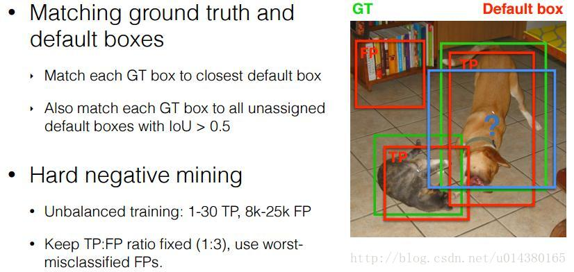
Matching strategy：

缩进在训练时，groundtruth boxes 与 default boxes（就是prior boxes）按照如下方式进行配对：

首先，寻找与每一个ground truth box有最大的jaccard overlap的default box，这样就能保证每一个groundtruth box与唯一的一个default box对应起来（所谓的jaccard overlap就是IoU，如图8）。
SSD之后又将剩余还没有配对的default box与任意一个groundtruth box尝试配对，只要两者之间的jaccard overlap大于阈值，就认为match（SSD 300 阈值为0.5）。
显然配对到GT的default box就是positive，没有配对到GT的default box就是negative。

图8 jaccard overlap

Hard negative mining：

缩进值得注意的是，一般情况下negative default boxes数量>>positive default boxes数量，直接训练会导致网络过于重视负样本，从而loss不稳定。所以需要采取：

所以SSD在训练时会依据confidience score排序default box，挑选其中confidience高的box进行训练，控制positive：negative=1：3

Data augmentation：

缩进数据增广，即每一张训练图像，随机的进行如下几种选择：

使用原始的图像
采样一个 patch，与物体之间最小的 jaccard overlap 为：0.1，0.3，0.5，0.7 或 0.9
随机的采样一个 patch

采样的 patch 是原始图像大小比例是[0.1，1]，aspect ratio在1/2与2之间。当 groundtruth box 的中心（center）在采样的patch中时，保留重叠部分。在这些采样步骤之后，每一个采样的patch被resize到固定的大小，并且以0.5的概率随机的水平翻转（horizontally flipped）。

其实Matching strategy，Hard negative mining，Data augmentation，都是为了加快网络收敛而设计的。尤其是Data augmentation，翻来覆去的randomly crop，保证每一个prior box都获得充分训练而已。不过当数据达到一定量的时候，不建议再进行Data augmentation，毕竟“真”的数据比“假”数据还是要好很多。

以ResNet作为前缀网络的SSD

http://blog.csdn.net/zhangjunbob/article/details/53119959

前面的部分直接使用ResNet网络即可，并且可以事先使用对应的数据集对ResNet网络进行预训练，后续直接将其接入SSD框架中，下面讲的是将ResNet50接入SSD中，对应的接入部分列出如下：

//至此resnet主体结构完成，随后接上ssd的结构

//用pool5作为bottom分别产生mbox_loc/mbox_conf/mbox_priorbox

layer {
  name: "pool5_mbox_loc"
  type: "Convolution"
  bottom: "pool5"                               //选取pool5作为bottom，产生mbox_loc
  top: "pool5_mbox_loc"
  param {
    lr_mult: 1
    decay_mult: 1
  }
  param {
    lr_mult: 2
    decay_mult: 0
  }
  convolution_param {
    num_output: 24
    pad: 1
    kernel_size: 3
    stride: 1
    weight_filler {
      type: "xavier"
    }
    bias_filler {
      type: "constant"
      value: 0
    }
  }
}
layer {
  name: "pool5_mbox_loc_perm"                     //将上一层产生的mbox_loc重新排序
  type: "Permute"
  bottom: "pool5_mbox_loc"
  top: "pool5_mbox_loc_perm"
  permute_param {
    order: 0
    order: 2
    order: 3
    order: 1
  }
}
layer {
  name: "pool5_mbox_loc_flat"                    //将上一层展平（例如7*7的展平成1*49，方便之后的拼接）
  type: "Flatten"
  bottom: "pool5_mbox_loc_perm"
  top: "pool5_mbox_loc_flat"
  flatten_param {
    axis: 1
  }
}
layer {
  name: "pool5_mbox_conf"
  type: "Convolution"
  bottom: "pool5"                               //选取pool5作为bottom，产生mbox_conf（之后的排序展平同理）
  top: "pool5_mbox_conf"
 param {
    lr_mult: 1
    decay_mult: 1
  }
  param {
    lr_mult: 2
    decay_mult: 0
  }
  convolution_param {
    num_output: 126
    pad: 1
    kernel_size: 3
    stride: 1
    weight_filler {
      type: "xavier"
    }
    bias_filler {
      type: "constant"
      value: 0
    }
  }
}
layer {
  name: "pool5_mbox_conf_perm"
  type: "Permute"
  bottom: "pool5_mbox_conf"
  top: "pool5_mbox_conf_perm"
  permute_param {
    order: 0
    order: 2
    order: 3
    order: 1
  }
}
layer {
  name: "pool5_mbox_conf_flat"
  type: "Flatten"
  bottom: "pool5_mbox_conf_perm"
  top: "pool5_mbox_conf_flat"
  flatten_param {
    axis: 1
  }
}
layer {
  name: "pool5_mbox_priorbox"
  type: "PriorBox"
  bottom: "pool5"                                //选取pool5作为bottom，产生mbox_priorbox（之后排序展平）
  bottom: "data"
  top: "pool5_mbox_priorbox"
  prior_box_param {
    min_size: 276.0
    max_size: 330.0
    aspect_ratio: 2
    aspect_ratio: 3
    flip: true
    clip: true
    variance: 0.1
    variance: 0.1
    variance: 0.2
    variance: 0.2
  }
}

//同理用res5c作为bottom分别产生mbox_loc/mbox_conf/mbox_priorbox

layer {
  name: "res5c_mbox_loc"
  type: "Convolution"
  bottom: "res5c"
  top: "res5c_mbox_loc"                                         
  param {
    lr_mult: 1
    decay_mult: 1
  }
  param {
    lr_mult: 2
    decay_mult: 0
  }
  convolution_param {
    num_output: 24
    pad: 1
    kernel_size: 3
    stride: 1
    weight_filler {
      type: "xavier"
    }
    bias_filler {
      type: "constant"
      value: 0
    }
  }
}
layer {
  name: "res5c_mbox_loc_perm"
  type: "Permute"
  bottom: "res5c_mbox_loc"
  top: "res5c_mbox_loc_perm"
  permute_param {
    order: 0
    order: 2
    order: 3
    order: 1
  }
}
layer {
  name: "res5c_mbox_loc_flat"
  type: "Flatten"
  bottom: "res5c_mbox_loc_perm"
  top: "res5c_mbox_loc_flat"
  flatten_param {
    axis: 1
  }
}
layer {
  name: "res5c_mbox_conf"
  type: "Convolution"
  bottom: "res5c"
  top: "res5c_mbox_conf"
  param {
    lr_mult: 1
    decay_mult: 1
  }
  param {
    lr_mult: 2
    decay_mult: 0
  }
  convolution_param {
    num_output: 126
    pad: 1
    kernel_size: 3
    stride: 1
    weight_filler {
      type: "xavier"
    }
    bias_filler {
      type: "constant"
      value: 0
    }
  }
}
layer {
  name: "res5c_mbox_conf_perm"
  type: "Permute"
  bottom: "res5c_mbox_conf"
  top: "res5c_mbox_conf_perm"
  permute_param {
    order: 0
    order: 2
    order: 3
    order: 1
  }
}
layer {
  name: "res5c_mbox_conf_flat"
  type: "Flatten"
  bottom: "res5c_mbox_conf_perm"
  top: "res5c_mbox_conf_flat"
  flatten_param {
    axis: 1
  }
}
layer {
  name: "res5c_mbox_priorbox"
  type: "PriorBox"
  bottom: "res5c"
  bottom: "data"
  top: "res5c_mbox_priorbox"
  prior_box_param {
    min_size: 276.0
    max_size: 330.0
    aspect_ratio: 2
    aspect_ratio: 3
    flip: true
    clip: true
    variance: 0.1
    variance: 0.1
    variance: 0.2
    variance: 0.2
  }
}


//Concat层将刚才的res5c和pool5产生的mbox_loc/mbox_conf/mbox_priorbox拼接起来形成一个层

layer {
  name: "mbox_loc"
  type: "Concat"
  bottom: "res5c_mbox_loc_flat"
  bottom: "pool5_mbox_loc_flat"
  top: "mbox_loc"
  concat_param {
    axis: 1
  }
}
layer {
  name: "mbox_conf"
  type: "Concat"
  bottom: "res5c_mbox_conf_flat"
  bottom: "pool5_mbox_conf_flat"
  top: "mbox_conf"
  concat_param {
    axis: 1
  }
}
layer {
  name: "mbox_priorbox"
  type: "Concat"
  bottom: "res5c_mbox_priorbox"
  bottom: "pool5_mbox_priorbox"
  top: "mbox_priorbox"
  concat_param {
    axis: 2
  }
}

<span style="color:#ff0000;">//mbox_loc,mbox_conf,mbox_priorbox一起做的loss-function</span>

layer {
  name: "mbox_loss"
  type: "MultiBoxLoss"
  bottom: "mbox_loc"
  bottom: "mbox_conf"
  bottom: "mbox_priorbox"
  bottom: "label"
  top: "mbox_loss"
  include {
    phase: TRAIN
  }
  propagate_down: true
  propagate_down: true
  propagate_down: false
  propagate_down: false
  loss_param {
    normalization: VALID
  }
  multibox_loss_param {
    loc_loss_type: SMOOTH_L1
    conf_loss_type: SOFTMAX
    loc_weight: 1.0
    num_classes: 21
    share_location: true
    match_type: PER_PREDICTION
    overlap_threshold: 0.5
    use_prior_for_matching: true
    background_label_id: 0
    use_difficult_gt: true
    do_neg_mining: true
    neg_pos_ratio: 3.0
    neg_overlap: 0.5
    code_type: CENTER_SIZE
  }
}

查看全文

相关阅读:
python文本处理
 转 Deep Learning for NLP 文章列举
 backpropagation
开发者必备的6款源码搜索引擎转
 转【面向代码】学习 Deep Learning（二）Deep Belief Nets(DBNs)
Sampling
各种形式的熵函数，KL距离
 [转] 如何在ie11里使用a连接创建动态下载文件流
 修改chrome背景色
 [转] 使用 Spring 5 的 WebFlux 开发反应式 Web 应用

原文地址：https://www.cnblogs.com/hansjorn/p/7445411.html