『科学计算』通过代码理解线性回归&Logistic回归模型

sklearn线性回归模型

import numpy as np
import matplotlib.pyplot as plt
from sklearn import linear_model

def get_data():
    #506行,14列，最后一列为label，前面13列为参数
    data_original = np.loadtxt('housing.data')  

    scale_data = scale_n(data_original)
    np.random.shuffle(scale_data)
    #在位置0，插入一列1，axis=1代表列，代表b
    data = np.insert(scale_data, 0, 1, axis=1) 

    train_X = data[:400, :-1] #前400行为训练数据
    train_y = data[:400, -1]
    train_y.shape = (train_y.shape[0],1)

    test_X = data[400:, :-1]
    test_y = data[400:, -1]
    test_y.shape = (test_y.shape[0],1)



    # test测试数据没有返回
    return train_X,train_y,test_X,test_y

def scale_n(x):
    return (x-x.mean(axis=0))/x.std(axis=0)


if __name__=="__main__":
    train_X,train_y,test_X,test_y = get_data()
    
    l_model = linear_model.Ridge(alpha = 1000)     # 参数是正则化系数
        
    l_model.fit(train_X,train_y)
    
    predict_train_y = l_model.predict(train_X)

    predict_train_y.shape = (predict_train_y.shape[0],1)
    error = (predict_train_y-train_y)
    rms_train = np.sqrt(np.mean(error**2, axis=0))        
    
    predict_test_y = l_model.predict(test_X)
    predict_test_y.shape = (predict_test_y.shape[0],1)
    error = (predict_test_y-test_y)
    rms_test = np.sqrt(np.mean(error**2, axis=0))
    
    print (rms_train, rms_test)
    
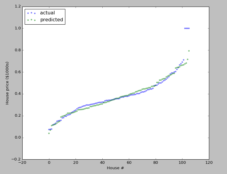
    plt.figure(figsize=(10, 8))
    plt.scatter(np.arange(test_y.size), sorted(test_y), c='b', edgecolor='None', alpha=0.5, label='actual')
    plt.scatter(np.arange(test_y.size), sorted(predict_test_y), c='g', edgecolor='None', alpha=0.5, label='predicted')
    plt.legend(loc='upper left')
    plt.ylabel('House price ($1000s)')
    plt.xlabel('House #')
    plt.show()

 sklearn模型调用民工三连：

l_model = linear_model.Ridge(alpha = 1000)     # 模型装载
        
l_model.fit(train_X,train_y)                   # 模型训练
    
predict_train_y = l_model.predict(train_X)     # 模型预测

手动线性回归模型

数据获取

房价数据，506行,14列，最后一列为label，前面13列为参数

假如我们需要平方特征，只要修改get_data()中的data_original即可，在13列后添加平方项或者立方项等，由于我们不知道具体添加多少特征的组合更好，神经网络自动提取组合特征的功能就被很好的凸显出来了

import numpy as np
import matplotlib.pyplot as plt

def get_data():
    #506行,14列，最后一列为label，前面13列为参数
    data_original = np.loadtxt('housing.data')      # 读取数据

    scale_data = scale_n(data_original)             # 归一化处理
    np.random.shuffle(scale_data)                   # 打乱顺序
    #在位置0，插入一列1，axis=1代表列，代表b
    data = np.insert(scale_data, 0, 1, axis=1)      # 数组插入函数


    train_X = data[:400, :-1]                       #前400行为训练数据
    train_y = data[:400, -1]
    train_y.shape = (train_y.shape[0],1)

    test_X = data[400:, :-1]
    test_y = data[400:, -1]
    test_y.shape = (test_y.shape[0],1)

    # test测试数据没有返回
    return train_X,train_y,test_X,test_y

其中：

np.loadtxt('housing.data')     # 读取数据
# 本函数读取数据后自动转化为ndarray数组，可以自行设定分隔符delimiter=","

np.insert(scale_data, 0, 1, axis=1)      # 数组插入函数

# 在数组中插入指定的行列，numpy.insert(arr, obj, values, axis=None）
# 和其他数组一样，axis不设定的话会把数组定为一维后插入，axis=0的话行扩展，axis=1的话列扩展

预处理

中心归零，标准差归一

def scale_n(x):
    """
    减去平均值，除以标准差
    """
    x = (x - np.mean(x,axis=0))/np.std(x,axis=0)
    return x

线性回归类

class LinearModel():
    def __init__(self,learn_rate=0.06,lamda=0.01,threhold=0.0000005):
        """
        初始化一些参数
        """
        self.learn_rate = learn_rate  # 学习率
        self.lamda = lamda            # 正则化系数
        self.threhold = threhold      # 迭代阈值
    
    def get_cost_grad(self,theta,X,y):
        """
        计算代价cost和梯度grad
        """
        y_pre = X.dot(theta)
        cost = (y_pre-y).T.dot(y_pre-y) + self.lamda*theta.T.dot(theta)
        grad = (2.0*X.T.dot(y_pre-y) + 2.0*self.lamda*theta)/X.shape[0]               # 实际上是1个batch的梯度的累加值
        return cost, grad
        
    def grad_check(self,X,y):
        """
        梯度检查： 函数计算梯度 == L(theta+delta)-L(theta-delta) / 2delta
        """
        m,n = X.shape
        delta = 10**(-4)
        sum_error = 0

        for i in range(100):
            theta = np.random.random((n,1))
            j = np.random.randint(1,n)

            theta1,theta2 = theta.copy(),theta.copy()
            theta1[j] += delta
            theta2[j] -= delta

            cost1, grad1 = self.get_cost_grad(theta1, X, y)
            cost2, grad2 = self.get_cost_grad(theta2, X, y)
            cost,  grad  = self.get_cost_grad(theta , X, y)

            sum_error += np.abs(grad[j] - (cost1-cost2)/(delta*2))
        print(sum_error/300.0)


    def train(self,X,y):
        """
        初始化theta
        训练后，将theta保存到实例变量里
        """
        m,n = X.shape
        theta = np.random.random((n,1))

        prev_cost = None
        for loop in range(1000):
            cost,grad = self.get_cost_grad(theta,X,y)
            theta -= self.learn_rate*grad
            if prev_cost:
                if prev_cost - cost < self.threhold:
                    break
            prev_cost = cost
        self.theta = theta
        # print(theta,loop,cost)


    def predict(self,X):
        """
        预测程序
        """
        return X.dot(self.theta)

 主函数

if __name__ == "__main__":
    train_X,train_y,test_X,test_y = get_data()

    linear_model = LinearModel()

    linear_model.grad_check(train_X,train_y)

    linear_model.train(train_X,train_y)

    predict_train_y = linear_model.predict(train_X)
    error = (predict_train_y - train_y)
    rms_train = np.sqrt(np.mean(error ** 2,axis=0))

    predict_test_y = linear_model.predict(test_X)
    error = (predict_test_y - test_y)
    rms_test = np.sqrt(np.mean(error ** 2,axis=0))
    #
    print(rms_train,rms_test)
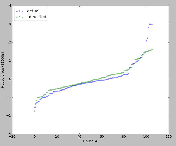
    # [ 0.54031084] [ 0.60065021]

    plt.figure(figsize=(10,8))
    plt.scatter(np.arange(test_y.size),sorted(test_y),c='b',edgecolor='None',alpha=0.5,label='actual')
    plt.scatter(np.arange(test_y.size),sorted(predict_test_y),c='g',edgecolor='None',alpha=0.5,label='predicted')
    plt.legend(loc='upper left')
    plt.ylabel('House price ($1000s)')
    plt.xlabel('House #')
    plt.show()

Logistic回归

数据获取&预处理

logistic回归输出值在0~1之间，所以数据预处理分两部分，前13列仍然是均值归零标准差归一，label列采取(x-x.min(axis=0))/(x.max(axis=0)-x.min(axis=0))的方式

import numpy as np
import matplotlib.pyplot as plt
import math

def get_data(N=400):
    #506行,14列，最后一列为label，前面13列为参数
    data_original = np.loadtxt('housing.data')  

    scale_data = np.zeros(data_original.shape)

    scale_data[:,:13] = scale_n(data_original[:,:13])
    scale_data[:,-1] = scale_max(data_original[:,-1])

    np.random.shuffle(scale_data)
    #在位置0，插入一列1，axis=1代表列，代表b
    data = np.insert(scale_data, 0, 1, axis=1) 

    train_X = data[:N, :-1] #前400行为训练数据
    train_y = data[:N, -1]
    train_y.shape = (train_y.shape[0],1)

    test_X = data[N:, :-1]
    test_y = data[N:, -1]
    test_y.shape = (test_y.shape[0],1)


    # test测试数据没有返回
    return train_X,train_y,test_X,test_y

def scale_n(x):
    return (x-x.mean(axis=0))/x.std(axis=0)
def scale_max(x):
    print (x.min(axis=0))
    print (x.max(axis=0))
    print (x.mean(axis=0))
    print (x.std(axis=0))

    return (x-x.min(axis=0))/(x.max(axis=0)-x.min(axis=0))

 Logistic回归类

 公式参考，

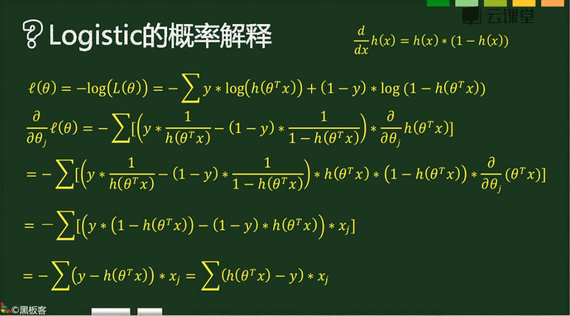
实际代码，

class LogisticModel(object):
    def __init__(self,lamda=0.01, alpha=0.6,threhold=0.0000005):
        self.alpha = alpha
        self.threhold = threhold
        self.lamda = lamda
        
    def sigmoid(self,x):
        return 1.0/(1+np.exp(-x))
        
    def get_cost_grad(self,theta,X,y):
        m, n = X.shape
        y_dash = self.sigmoid(X.dot(theta))
        error = np.sum((y * np.log(y_dash) + (1-y) * np.log(1-y_dash)),axis=1)
        cost = -np.sum(error, axis=0)+self.lamda*theta.T.dot(theta)
        grad = X.T.dot(y_dash-y)+2.0*self.lamda*theta
                    
        return cost,grad/m
        
        
    def grad_check(self,X,y):
        epsilon = 10**-4
        m, n = X.shape   
        
        sum_error=0
        
        for i in range(300):
            theta = np.random.random((n, 1))
            j = np.random.randint(1,n)
            theta1=theta.copy()
            theta2=theta.copy()
            theta1[j]+=epsilon
            theta2[j]-=epsilon

            cost1,grad1 = self.get_cost_grad(theta1,X,y)
            cost2,grad2 = self.get_cost_grad(theta2,X,y)
            cost3,grad3 = self.get_cost_grad(theta,X,y)

            sum_error += np.abs(grad3[j]-(cost1-cost2)/float(2*epsilon))
        
    def train(self,X,y):
        m, n = X.shape  # 400,15   
        theta = np.random.random((n, 1))  #[15,1]
        #our intial prediction
        prev_cost = None
        loop_num = 0
        while(True):                      

            #intial cost
            cost,grad = self.get_cost_grad(theta,X,y)
            
            theta = theta- self.alpha * grad
            
            loop_num+=1
            if loop_num%100==0:
                print (cost,loop_num)
            if prev_cost:
                if prev_cost - cost <= self.threhold:
                    break
            if loop_num>1000:
                break

            prev_cost = cost
                       
            
        self.theta = theta
        print (theta,loop_num)
        
    def predict(self,X):
        return self.sigmoid(X.dot(self.theta))