集成学习和代码实现

从百度云课堂上截图的基础概念，如果之前不了解的可以先看一下这篇博客：https://blog.csdn.net/weixin_30708329/article/details/97262409

 

 

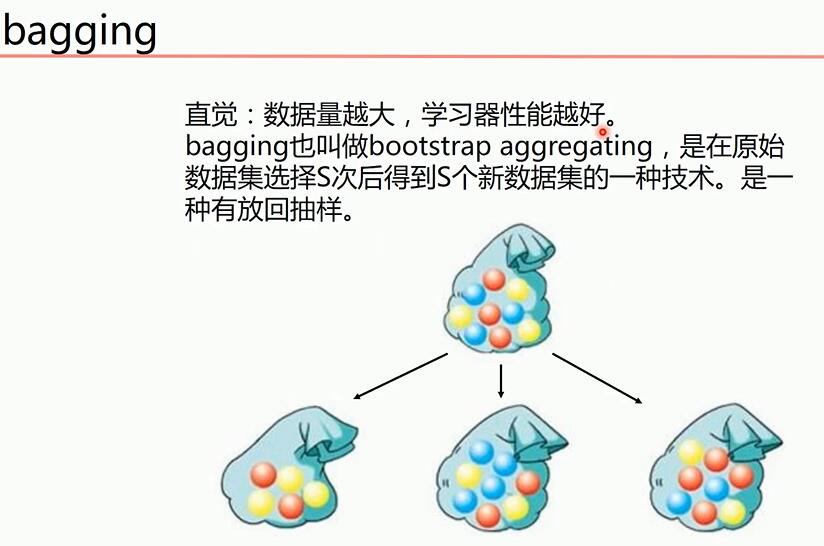
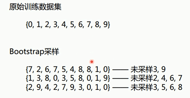
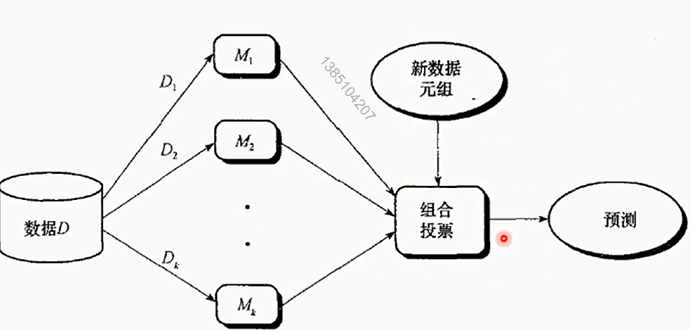
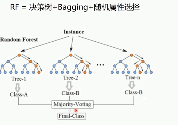
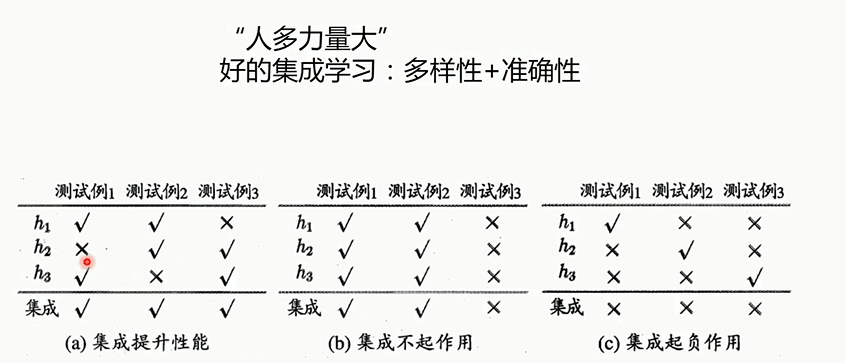
不同的数据集训练不同的模型，根据模型进行投票得到最终预测结果

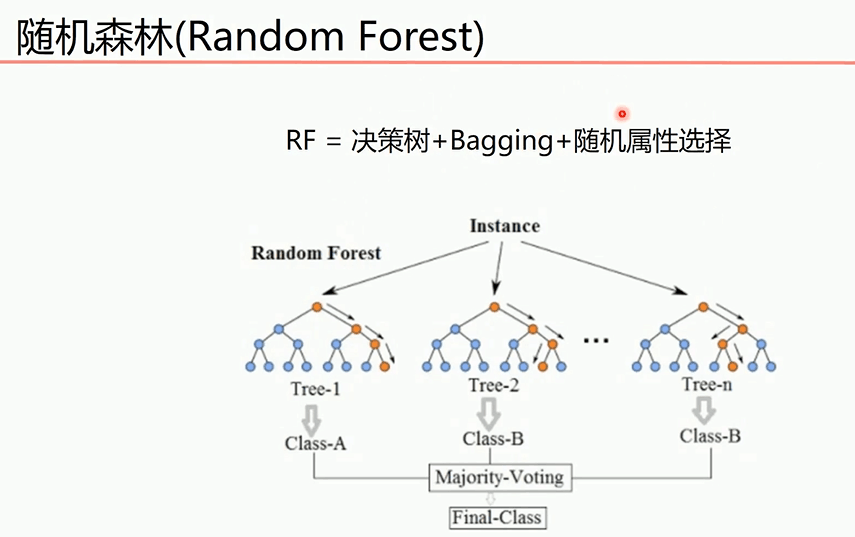
多棵决策树组成森林，每个模型训练集不同和选择的决策属性不同是RF算法随机的最主要体现

 

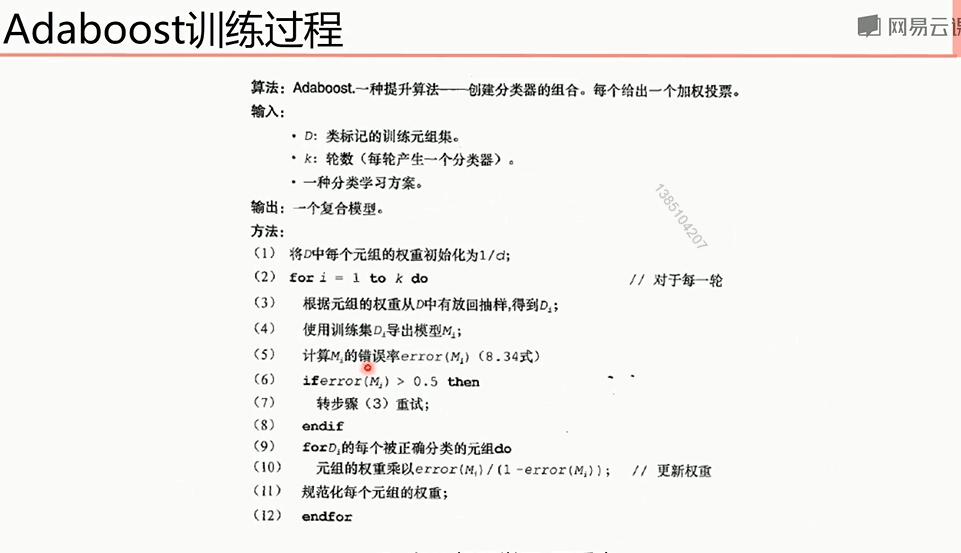
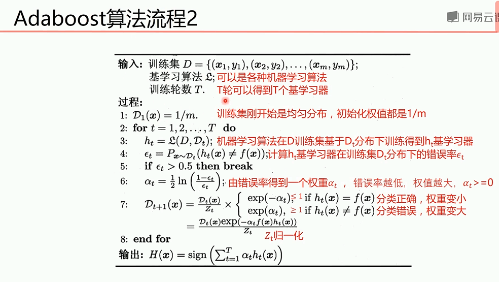
adaboost算法不同模型之间会有影响

 

 

 

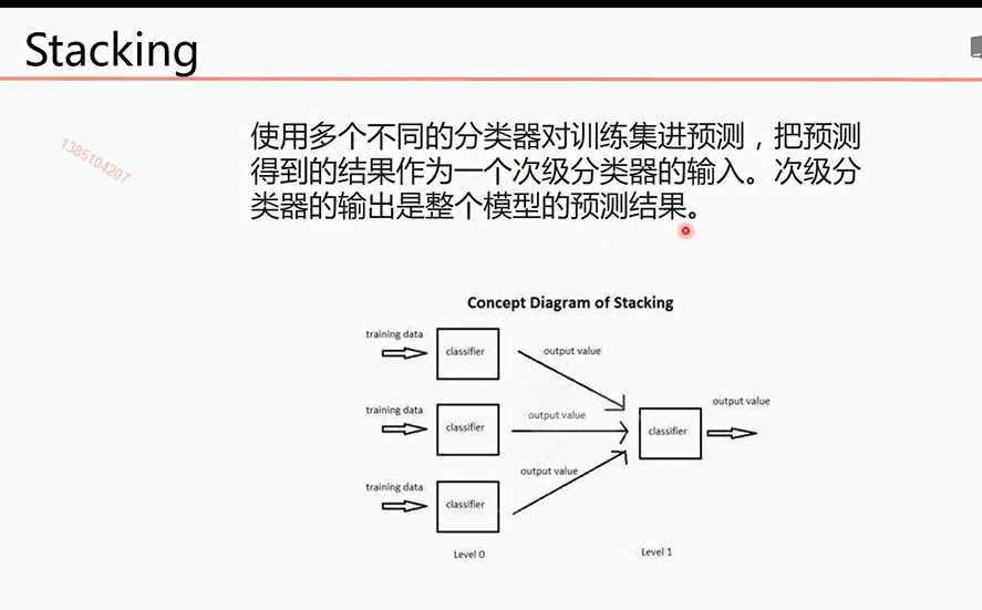
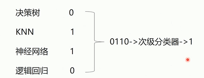
多层分类器进行结果的预测

 bagging算法提高KNN和决策树算法精确度

# 导入算法包以及数据集
from sklearn import neighbors
from sklearn import datasets
from sklearn.ensemble import BaggingClassifier
from sklearn import tree
from sklearn.model_selection import train_test_split
import numpy as np
import matplotlib.pyplot as plt
iris = datasets.load_iris()
x_data = iris.data[:,:2]
y_data = iris.target
def plot(model):
    # 获取数据值所在的范围
    x_min, x_max = x_data[:, 0].min() - 1, x_data[:, 0].max() + 1
    y_min, y_max = x_data[:, 1].min() - 1, x_data[:, 1].max() + 1

    # 生成网格矩阵
    xx, yy = np.meshgrid(np.arange(x_min, x_max, 0.02),
                         np.arange(y_min, y_max, 0.02))

    z = model.predict(np.c_[xx.ravel(), yy.ravel()])# ravel与flatten类似，多维数据转一维。flatten不会改变原始数据，ravel会改变原始数据
    z = z.reshape(xx.shape)
    # 等高线图
    cs = plt.contourf(xx, yy, z)
x_train,x_test,y_train,y_test = train_test_split(x_data, y_data)
knn = neighbors.KNeighborsClassifier()
knn.fit(x_train, y_train)
# 画图
plot(knn)
# 样本散点图
plt.scatter(x_data[:, 0], x_data[:, 1], c=y_data)
plt.show()
# 准确率
print("knn:",knn.score(x_test, y_test))
dtree = tree.DecisionTreeClassifier()
dtree.fit(x_train, y_train)
# 画图
plot(dtree)
# 样本散点图
plt.scatter(x_data[:, 0], x_data[:, 1], c=y_data)
plt.show()
# 准确率
print("dtree:",dtree.score(x_test, y_test))
bagging_knn = BaggingClassifier(knn, n_estimators=100)#使用bagging算法训练100组knn分类器
# 输入数据建立模型
bagging_knn.fit(x_train, y_train)
plot(bagging_knn)
# 样本散点图
plt.scatter(x_data[:, 0], x_data[:, 1], c=y_data)
plt.show()
print("bagging:",bagging_knn.score(x_test, y_test))
bagging_tree = BaggingClassifier(dtree, n_estimators=100)#使用bagging算法训练100组决策树分类器
# 输入数据建立模型
bagging_tree.fit(x_train, y_train)
plot(bagging_tree)
# 样本散点图
plt.scatter(x_data[:, 0], x_data[:, 1], c=y_data)
plt.show()
print("bagging_tree",bagging_tree.score(x_test, y_test))

随机森林对决策树模型优化

from sklearn import tree
from sklearn.model_selection import train_test_split
from sklearn.ensemble import RandomForestClassifier
import numpy as np
import matplotlib.pyplot as plt
# 载入数据
data = np.genfromtxt("LR-testSet2.txt", delimiter=",")
x_data = data[:,:-1]
y_data = data[:,-1]

plt.scatter(x_data[:,0],x_data[:,1],c=y_data)
plt.show()
x_train,x_test,y_train,y_test = train_test_split(x_data, y_data, test_size = 0.5)
def plot(model):
    # 获取数据值所在的范围
    x_min, x_max = x_data[:, 0].min() - 1, x_data[:, 0].max() + 1
    y_min, y_max = x_data[:, 1].min() - 1, x_data[:, 1].max() + 1

    # 生成网格矩阵
    xx, yy = np.meshgrid(np.arange(x_min, x_max, 0.02),
                         np.arange(y_min, y_max, 0.02))

    z = model.predict(np.c_[xx.ravel(), yy.ravel()])# ravel与flatten类似，多维数据转一维。flatten不会改变原始数据，ravel会改变原始数据
    z = z.reshape(xx.shape)
    # 等高线图
    cs = plt.contourf(xx, yy, z)
    # 样本散点图
    plt.scatter(x_test[:, 0], x_test[:, 1], c=y_test)
    plt.show()
dtree = tree.DecisionTreeClassifier()
dtree.fit(x_train, y_train)
plot(dtree)
print("dtree",dtree.score(x_test, y_test))
RF = RandomForestClassifier(n_estimators=50)
RF.fit(x_train, y_train)
plot(RF)
print("RandomForest",RF.score(x_test, y_test))

下面是用到的数据

0.051267,0.69956,1
-0.092742,0.68494,1
-0.21371,0.69225,1
-0.375,0.50219,1
-0.51325,0.46564,1
-0.52477,0.2098,1
-0.39804,0.034357,1
-0.30588,-0.19225,1
0.016705,-0.40424,1
0.13191,-0.51389,1
0.38537,-0.56506,1
0.52938,-0.5212,1
0.63882,-0.24342,1
0.73675,-0.18494,1
0.54666,0.48757,1
0.322,0.5826,1
0.16647,0.53874,1
-0.046659,0.81652,1
-0.17339,0.69956,1
-0.47869,0.63377,1
-0.60541,0.59722,1
-0.62846,0.33406,1
-0.59389,0.005117,1
-0.42108,-0.27266,1
-0.11578,-0.39693,1
0.20104,-0.60161,1
0.46601,-0.53582,1
0.67339,-0.53582,1
-0.13882,0.54605,1
-0.29435,0.77997,1
-0.26555,0.96272,1
-0.16187,0.8019,1
-0.17339,0.64839,1
-0.28283,0.47295,1
-0.36348,0.31213,1
-0.30012,0.027047,1
-0.23675,-0.21418,1
-0.06394,-0.18494,1
0.062788,-0.16301,1
0.22984,-0.41155,1
0.2932,-0.2288,1
0.48329,-0.18494,1
0.64459,-0.14108,1
0.46025,0.012427,1
0.6273,0.15863,1
0.57546,0.26827,1
0.72523,0.44371,1
0.22408,0.52412,1
0.44297,0.67032,1
0.322,0.69225,1
0.13767,0.57529,1
-0.0063364,0.39985,1
-0.092742,0.55336,1
-0.20795,0.35599,1
-0.20795,0.17325,1
-0.43836,0.21711,1
-0.21947,-0.016813,1
-0.13882,-0.27266,1
0.18376,0.93348,0
0.22408,0.77997,0
0.29896,0.61915,0
0.50634,0.75804,0
0.61578,0.7288,0
0.60426,0.59722,0
0.76555,0.50219,0
0.92684,0.3633,0
0.82316,0.27558,0
0.96141,0.085526,0
0.93836,0.012427,0
0.86348,-0.082602,0
0.89804,-0.20687,0
0.85196,-0.36769,0
0.82892,-0.5212,0
0.79435,-0.55775,0
0.59274,-0.7405,0
0.51786,-0.5943,0
0.46601,-0.41886,0
0.35081,-0.57968,0
0.28744,-0.76974,0
0.085829,-0.75512,0
0.14919,-0.57968,0
-0.13306,-0.4481,0
-0.40956,-0.41155,0
-0.39228,-0.25804,0
-0.74366,-0.25804,0
-0.69758,0.041667,0
-0.75518,0.2902,0
-0.69758,0.68494,0
-0.4038,0.70687,0
-0.38076,0.91886,0
-0.50749,0.90424,0
-0.54781,0.70687,0
0.10311,0.77997,0
0.057028,0.91886,0
-0.10426,0.99196,0
-0.081221,1.1089,0
0.28744,1.087,0
0.39689,0.82383,0
0.63882,0.88962,0
0.82316,0.66301,0
0.67339,0.64108,0
1.0709,0.10015,0
-0.046659,-0.57968,0
-0.23675,-0.63816,0
-0.15035,-0.36769,0
-0.49021,-0.3019,0
-0.46717,-0.13377,0
-0.28859,-0.060673,0
-0.61118,-0.067982,0
-0.66302,-0.21418,0
-0.59965,-0.41886,0
-0.72638,-0.082602,0
-0.83007,0.31213,0
-0.72062,0.53874,0
-0.59389,0.49488,0
-0.48445,0.99927,0
-0.0063364,0.99927,0
0.63265,-0.030612,0

adaboost决策树

import numpy as np
import matplotlib.pyplot as plt
from sklearn import tree
from sklearn.ensemble import AdaBoostClassifier
from sklearn.tree import DecisionTreeClassifier
from sklearn.datasets import make_gaussian_quantiles
from sklearn.metrics import classification_report
# 生成2维正态分布，生成的数据按分位数分为两类，500个样本,2个样本特征
x1, y1 = make_gaussian_quantiles(n_samples=500, n_features=2,n_classes=2)#默认mean=(0, 0)
# 生成2维正态分布，生成的数据按分位数分为两类，400个样本,2个样本特征均值都为3
x2, y2 = make_gaussian_quantiles(mean=(3, 3), n_samples=500, n_features=2, n_classes=2)
# 将两组数据合成一组数据
x_data = np.concatenate((x1, x2))
y_data = np.concatenate((y1, - y2 + 1))
plt.scatter(x_data[:, 0], x_data[:, 1], c=y_data)
plt.show()
# 决策树模型
model = tree.DecisionTreeClassifier(max_depth=3)

# 输入数据建立模型
model.fit(x_data, y_data)

# 获取数据值所在的范围
x_min, x_max = x_data[:, 0].min() - 1, x_data[:, 0].max() + 1
y_min, y_max = x_data[:, 1].min() - 1, x_data[:, 1].max() + 1

# 生成网格矩阵
xx, yy = np.meshgrid(np.arange(x_min, x_max, 0.02),
                     np.arange(y_min, y_max, 0.02))

z = model.predict(np.c_[xx.ravel(), yy.ravel()])# ravel与flatten类似，多维数据转一维。flatten不会改变原始数据，ravel会改变原始数据
z = z.reshape(xx.shape)
# 等高线图
cs = plt.contourf(xx, yy, z)
# 样本散点图
plt.scatter(x_data[:, 0], x_data[:, 1], c=y_data)
plt.show()
# 模型准确率
print("决策树：",model.score(x_data,y_data))
# AdaBoost模型
model = AdaBoostClassifier(DecisionTreeClassifier(max_depth=3),n_estimators=10)#决策树深度为3，一共训练十个模型
# 训练模型
model.fit(x_data, y_data)

# 获取数据值所在的范围
x_min, x_max = x_data[:, 0].min() - 1, x_data[:, 0].max() + 1
y_min, y_max = x_data[:, 1].min() - 1, x_data[:, 1].max() + 1

# 生成网格矩阵
xx, yy = np.meshgrid(np.arange(x_min, x_max, 0.02),
                     np.arange(y_min, y_max, 0.02))

# 获取预测值
z = model.predict(np.c_[xx.ravel(), yy.ravel()])
z = z.reshape(xx.shape)
# 等高线图
cs = plt.contourf(xx, yy, z)
# 样本散点图
plt.scatter(x_data[:, 0], x_data[:, 1], c=y_data)
plt.show()
# 模型准确率
print("adaboost：",model.score(x_data,y_data))#得分很高

stacking分类器算法

from sklearn import datasets
from sklearn import model_selection
from sklearn.linear_model import LogisticRegression
from sklearn.neighbors import KNeighborsClassifier
from sklearn.tree import DecisionTreeClassifier
from mlxtend.classifier import StackingClassifier # pip install mlxtend
import numpy as np

# 载入数据集
iris = datasets.load_iris()
# 只要第1,2列的特征
x_data, y_data = iris.data[:, 1:3], iris.target

# 定义三个不同的分类器
clf1 = KNeighborsClassifier(n_neighbors=1)
clf2 = DecisionTreeClassifier()
clf3 = LogisticRegression()

# 定义一个次级分类器
lr = LogisticRegression()
sclf = StackingClassifier(classifiers=[clf1, clf2, clf3],
                          meta_classifier=lr)

for clf, label in zip([clf1, clf2, clf3, sclf],
                      ['KNN', 'Decision Tree', 'LogisticRegression', 'StackingClassifier']):
    scores = model_selection.cross_val_score(clf, x_data, y_data, cv=3, scoring='accuracy')
    print("Accuracy: %0.2f [%s]" % (scores.mean(), label))

voting分类器

from sklearn import datasets
from sklearn import model_selection
from sklearn.linear_model import LogisticRegression
from sklearn.neighbors import KNeighborsClassifier
from sklearn.tree import DecisionTreeClassifier
from sklearn.ensemble import VotingClassifier
import numpy as np

# 载入数据集
iris = datasets.load_iris()
# 只要第1,2列的特征
x_data, y_data = iris.data[:, 1:3], iris.target

# 定义三个不同的分类器
clf1 = KNeighborsClassifier(n_neighbors=1)
clf2 = DecisionTreeClassifier()
clf3 = LogisticRegression()

sclf = VotingClassifier([('knn', clf1), ('dtree', clf2), ('lr', clf3)])

for clf, label in zip([clf1, clf2, clf3, sclf],
                      ['KNN', 'Decision Tree', 'LogisticRegression', 'VotingClassifier']):
    scores = model_selection.cross_val_score(clf, x_data, y_data, cv=3, scoring='accuracy')
    print("Accuracy: %0.2f [%s]" % (scores.mean(), label))