python 线性回归示例

说明：此文的第一部分参考了这里

用python进行线性回归分析非常方便，有现成的库可以使用比如：numpy.linalog.lstsq例子、scipy.stats.linregress例子、pandas.ols例子等。

不过本文使用sklearn库的linear_model.LinearRegression，支持任意维度，非常好用。

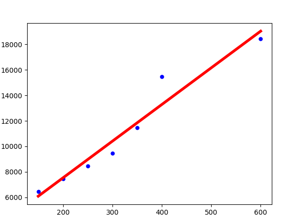
一、二维直线的例子

预备知识：线性方程(y = a * x + b) 表示平面一直线

下面的例子中，我们根据房屋面积、房屋价格的历史数据，建立线性回归模型。

然后，根据给出的房屋面积，来预测房屋价格。这里是数据来源

import pandas as pd
from io import StringIO

from sklearn import linear_model

import matplotlib.pyplot as plt



# 房屋面积与价格历史数据(csv文件)
csv_data = 'square_feet,price
150,6450
200,7450
250,8450
300,9450
350,11450
400,15450
600,18450
'

# 读入dataframe
df = pd.read_csv(StringIO(csv_data))
print(df)


# 建立线性回归模型
regr = linear_model.LinearRegression()

# 拟合
regr.fit(df['square_feet'].reshape(-1, 1), df['price']) # 注意此处.reshape(-1, 1)，因为X是一维的！

# 不难得到直线的斜率、截距
a, b = regr.coef_, regr.intercept_

# 给出待预测面积
area = 238.5

# 方式1：根据直线方程计算的价格
print(a * area + b)

# 方式2：根据predict方法预测的价格
print(regr.predict(area))

# 画图
# 1.真实的点
plt.scatter(df['square_feet'], df['price'], color='blue')

# 2.拟合的直线
plt.plot(df['square_feet'], regr.predict(df['square_feet'].reshape(-1,1)), color='red', linewidth=4)

plt.show()

效果图

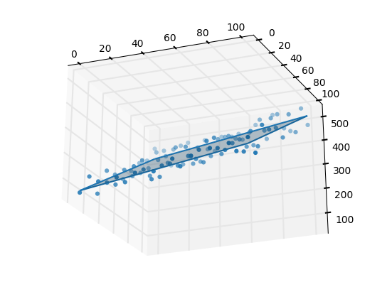
二、三维平面的例子

预备知识：线性方程(z = a * x + b * y + c) 表示空间一平面

由于找不到真实数据，只好自己虚拟一组数据。

import numpy as np

from sklearn import linear_model

from mpl_toolkits.mplot3d import Axes3D
import matplotlib.pyplot as plt


xx, yy = np.meshgrid(np.linspace(0,10,10), np.linspace(0,100,10))
zz = 1.0 * xx + 3.5 * yy + np.random.randint(0,100,(10,10))

# 构建成特征、值的形式
X, Z = np.column_stack((xx.flatten(),yy.flatten())), zz.flatten()

# 建立线性回归模型
regr = linear_model.LinearRegression()

# 拟合
regr.fit(X, Z)


# 不难得到平面的系数、截距
a, b = regr.coef_, regr.intercept_

# 给出待预测的一个特征
x = np.array([[5.8, 78.3]])

# 方式1：根据线性方程计算待预测的特征x对应的值z（注意：np.sum）
print(np.sum(a * x) + b)

# 方式2：根据predict方法预测的值z
print(regr.predict(x))


# 画图
fig = plt.figure()
ax = fig.gca(projection='3d')

# 1.画出真实的点
ax.scatter(xx, yy, zz)

# 2.画出拟合的平面
ax.plot_wireframe(xx, yy, regr.predict(X).reshape(10,10))
ax.plot_surface(xx, yy, regr.predict(X).reshape(10,10), alpha=0.3)


plt.show()

效果图