一、NumPy简介
Numpy中文网站:
https://www.numpy.org.cn/index.html
NumPy是使用Python进行科学计算的基本软件包。它包含以下内容:
-
强大的N维数组对象
-
复杂的(广播)功能
-
集成C / C ++和Fortran代码的工具
-
有用的线性代数,傅立叶变换和随机数功能
除了其明显的科学用途外,NumPy还可以用作通用数据的高效多维容器。可以定义任意数据类型。这使NumPy可以无缝,快速地与各种数据库集成。
NumPy包的核心是ndarray对象,n维数组,电脑上的所有数据都是数字形式保存
二、创建ndarray
1、使用np.array()由Python中的list创建
注意:
numpy默认ndarray的所有元素的类型是相同的
如果传进来的列表中包含不同的类型,则统一为同一类型,优先级:str>float>int
# 一维数组
>>>l = [1,2,3,4,5,6]
>>>l
[1,2,3,4,5,6]
>>>type(l)
list
>>>nd = np.array(l)
>>>nd
array([1, 2, 3, 4, 5, 6])
>>>type(nd)
numpy.ndarray

# 二维数组
>>>l2 = [[1,3,5,7],[2,4,6,8]]
>>>nd2 = np.array(l2)
>>>nd2
array([[1, 3, 5, 7],
       [2, 4, 6, 8]])
扩展:ndarray中的方法运行时间与Python自定义方法运行时间对比
使用ndarray中的方法
>>>x = np.arange(0,1000000,1)
>>>%timeit x.sum()    # %timeit在ipython的魔法方法,计算平均运行速度
7.49 µs ± 297 ns per loop (mean ± std. dev. of 7 runs, 100000 loops each)
使用Python自定义方法
>>> def sum2(x):
...:     ret=0
...:     for i in x:
...:         ret+=i
...:     return ret

>>> %timeit sum2(x)
943 µs ± 21.6 µs per loop (mean ± std. dev. of 7 runs, 1000 loops each)
2、使用np的routines函数创建
2.1、np.ones(shape,dtype=None, order='C')
>>>np.ones(shape=(5,5),dtype=np.int16)
array([[1, 1, 1, 1, 1],
       [1, 1, 1, 1, 1],
       [1, 1, 1, 1, 1],
       [1, 1, 1, 1, 1],
       [1, 1, 1, 1, 1]], dtype=int16)
2.2、np.zeros(shape, dtype=float,order='C')
>>>np.zeros(shape=(2,3,4),dtype=np.float16,order='C')
array([[[0., 0., 0., 0.],
        [0., 0., 0., 0.],
        [0., 0., 0., 0.]],

       [[0., 0., 0., 0.],
        [0., 0., 0., 0.],
        [0., 0., 0., 0.]]], dtype=float16)
2.3、np.full(shape,fill_value,dtype=None,order='C')
>>>np.full(shape=(3,5),fill_value=3.14)
array([[3.14, 3.14, 3.14, 3.14, 3.14],
       [3.14, 3.14, 3.14, 3.14, 3.14],
       [3.14, 3.14, 3.14, 3.14, 3.14]])
2.4、np.eye(N,M=None,k=0,dtype=float)
对角线为1,其他都为0(单位矩阵)
>>>np.eye(N=5)
array([[1., 0., 0., 0., 0.],
       [0., 1., 0., 0., 0.],
       [0., 0., 1., 0., 0.],
       [0., 0., 0., 1., 0.],
       [0., 0., 0., 0., 1.]])
2.5、np.linspace(start,stop,num=50,endpoint=True,retstep=False,dtype=None,axis=0)
等差数列,默认元素个数为50
>>>np.linspace(0,100,num=101)
array([  0.,   1.,   2.,   3.,   4.,   5.,   6.,   7.,   8.,   9.,  10.,
        11.,  12.,  13.,  14.,  15.,  16.,  17.,  18.,  19.,  20.,  21.,
        22.,  23.,  24.,  25.,  26.,  27.,  28.,  29.,  30.,  31.,  32.,
        33.,  34.,  35.,  36.,  37.,  38.,  39.,  40.,  41.,  42.,  43.,
        44.,  45.,  46.,  47.,  48.,  49.,  50.,  51.,  52.,  53.,  54.,
        55.,  56.,  57.,  58.,  59.,  60.,  61.,  62.,  63.,  64.,  65.,
        66.,  67.,  68.,  69.,  70.,  71.,  72.,  73.,  74.,  75.,  76.,
        77.,  78.,  79.,  80.,  81.,  82.,  83.,  84.,  85.,  86.,  87.,
        88.,  89.,  90.,  91.,  92.,  93.,  94.,  95.,  96.,  97.,  98.,
        99., 100.])
2.6、np.arange([start,]stop,[step,] dtype=None)
>>> np.arange(0, 100 , 3)

array([ 0,  3,  6,  9, 12, 15, 18, 21, 24, 27, 30, 33, 36, 39, 42, 45, 48,51, 54, 57, 60, 63, 66, 69, 72, 75, 78, 81, 84, 87, 90, 93, 96, 99])
2.7、np.random.randint(low, high=None, size=None, dtype='l')
size和shape一样,都表示形状
>>>np.random.randint(0,100,size=(5,5))
array([[74, 88, 31, 50, 86],
       [36, 30, 60, 82, 52],
       [75, 35, 13, 62, 56],
       [55, 81, 11, 31, 35],
       [70, 46, 37, 50, 15]])
2.8、np.random.randn(d0,d1,...,dn)
标准正太分步,平均值是0,方差是1(方差是指一组数据中的各个数减这组数据的平均数的平方和的平均数)
>>>np.random.randn(4,5)
array([[-0.65929266, -0.1158144 ,  1.46657156, -0.26807727, -0.53796907],
       [ 0.99267595,  0.3041624 ,  0.96071039,  0.14393343, -0.36095243],
       [-0.379658  ,  1.04786276,  0.59278064,  0.50335096, -0.3277399 ],
       [ 0.17712782,  1.23954189,  0.56248504, -1.99292278,  0.08521592]])
2.9、np.random.normal(loc=0.0,scale=1.0.size=None)
>>>nd = np.random.normal(loc=175,scale=10,size=100).round(2)
>>>nd
array([186.32, 166.21, 180.74, 165.06, 182.66, 170.81, 173.23, 176.29,
       170.76, 170.6 , 151.08, 176.12, 163.31, 191.16, 191.59, 164.01,
       183.78, 192.48, 175.52, 169.19, 164.42, 172.54, 172.58, 177.23,
       174.09, 187.7 , 179.62, 170.99, 161.09, 170.54, 193.89, 161.95,
       176.8 , 171.9 , 165.14, 177.63, 178.79, 165.54, 182.23, 188.34,
       188.56, 177.  , 183.04, 167.11, 177.26, 177.58, 173.  , 173.88,
       189.18, 188.02, 172.19, 165.96, 178.38, 177.95, 169.87, 184.81,
       197.21, 174.83, 160.56, 188.6 , 176.77, 171.17, 158.34, 186.84,
       180.35, 187.73, 173.72, 172.84, 173.95, 149.39, 170.18, 191.  ,
       176.08, 169.75, 185.91, 157.16, 174.65, 179.04, 175.75, 185.73,
       176.86, 174.97, 185.35, 166.77, 173.36, 177.17, 163.02, 168.31,
       157.95, 174.95, 184.31, 177.25, 187.86, 175.7 , 173.53, 183.81,
       162.49, 174.28, 178.86, 184.48])

>>>nd.mean()
175.56550000000004

>>>nd.var() # 方差
89.79609674999998

>>>nd.std()  # 标准差,是方差的开平方
9.476080241851056
3.0、np.random.random(size=None)
生成0到1的随机数,左闭右开
>>>np.random.random(100)
array([0.42394413, 0.39535747, 0.00117769, 0.06222843, 0.23552499,
       0.58703842, 0.41098732, 0.53515668, 0.38935586, 0.36003518,
       0.17040341, 0.9336931 , 0.36135176, 0.2581113 , 0.77797719,
       0.80391733, 0.57084769, 0.65220096, 0.71446975, 0.75216334,
       0.34995834, 0.2434726 , 0.46951549, 0.99420428, 0.28646191,
       0.29843906, 0.51456345, 0.76068483, 0.12516705, 0.09427598,
       0.49790385, 0.69853115, 0.05512114, 0.7181321 , 0.36524157,
       0.27626429, 0.85277254, 0.95415285, 0.22525194, 0.75216313,
       0.17002706, 0.6389772 , 0.51445091, 0.35205223, 0.60396478,
       0.56805125, 0.09502962, 0.65222939, 0.68848764, 0.75423821,
       0.14716734, 0.45095856, 0.26134085, 0.35042213, 0.63346907,
       0.36167779, 0.02816072, 0.11018343, 0.89248301, 0.06399121,
       0.69225864, 0.5668046 , 0.30777224, 0.8232473 , 0.29443376,
       0.56196357, 0.08535839, 0.14799983, 0.10439367, 0.99432287,
       0.10112337, 0.88614082, 0.99978457, 0.234225  , 0.31199546,
       0.69026256, 0.86672978, 0.97610685, 0.78551636, 0.26795029,
       0.56460585, 0.30096606, 0.078799  , 0.40604941, 0.05092757,
       0.0875861 , 0.03910609, 0.01884046, 0.97836117, 0.73813363,
       0.07438561, 0.7174979 , 0.13436745, 0.38924136, 0.96119282,
       0.11766203, 0.78268217, 0.30611418, 0.96945967, 0.8903713 ])
三、ndarray的属性
ndim:维度
shape:形状(各维度的长度)
size:总长度
dtype:元素类型
>>>nd = np.random.normal(loc=175,scale=10,size=100).round(2)
>>>nd
array([176.57, 172.91, 161.08, 168.89, 170.06, 156.68, 175.3 , 167.14,
       158.04, 170.64, 176.93, 190.66, 167.12, 175.89, 168.15, 178.26,
       184.91, 194.36, 163.35, 163.2 , 182.33, 192.39, 170.3 , 183.77,
       174.67, 171.13, 190.17, 171.64, 151.57, 182.94, 165.22, 183.78,
       172.88, 170.16, 177.49, 171.18, 171.37, 171.77, 179.39, 160.14,
       174.8 , 167.85, 187.41, 178.15, 191.68, 158.65, 169.78, 167.46,
       185.52, 169.97, 163.15, 149.73, 191.29, 181.93, 197.99, 169.65,
       186.89, 179.05, 175.32, 164.76, 172.85, 179.38, 169.89, 169.79,
       160.55, 173.62, 178.26, 185.48, 177.83, 179.98, 183.48, 170.1 ,
       168.07, 182.11, 166.5 , 172.86, 165.39, 176.21, 175.38, 169.49,
       184.47, 188.04, 169.98, 171.55, 178.78, 169.49, 171.27, 172.79,
       174.24, 176.48, 176.26, 170.03, 184.89, 201.49, 165.39, 172.42,
       170.25, 195.73, 173.31, 180.43])
1、size
>>>nd.size
100
2、shape
>>>nd.shape
(100,)
3、dtype
>>>nd.dtype
dtype('float64')
4、ndim
>>>nd.ndim
1
四、ndarray的基本操作
>>>nd2 = np.random.randint(0,150,size=(4,5))
>>>nd2
array([[ 65,  46, 121,  56,  17],
       [140, 141,  42,  53, 122],
       [ 44,  65,  74,  58,  43],
       [146,  51,  29,  69,  94]])
1、索引
一维与列表完全一致,多维时和一维二维规律完全一致,只是复杂度高一些
# 取出141,首先找出在哪一行,然后找出具体位置
>>>nd[1,1]
141
# 取出第三行整行数据
>>>nd2[2]
array([44, 65, 74, 58, 43])
2、切片
一维与列表完全一致,多维时同理
2.1获取前三行数据
>>>nd2[0:3]
array([[ 65,  46, 121,  56,  17],
       [140, 141,  42,  53, 122],
       [ 44,  65,  74,  58,  43]])
2.2获取最后两行数据
>>>nd2[-2:]
array([[ 44,  65,  74,  58,  43],
       [146,  51,  29,  69,  94]])
2.3获取最后两行以及最后两列数据
>>nd2[-2:,-2:]
array([[58, 43],
       [69, 94]])
2.4、将数据反转
>>>nd3 = np.random.randint(0,100,size=30)[:10]
>>>nd3
array([66, 85, 53,  2, 36, 24, 10, 70, 18, 49])

# 进行反转
>>>nd3[::-1]
array([49, 18, 70, 10, 24, 36,  2, 53, 85, 66])
2.5、两个::进行切片
>>>nd4 = np.random.randint(0,100,size=30)
>>>np4
array([55, 30, 16,  8, 61, 69, 70,  3, 60, 80, 82, 28,  3, 17, 53, 87,  2,
       62, 54, 49, 41, 90, 78, 90, 20, 23, 12, 99, 29, 31])

>>>nd4[::2]
array([55, 16, 61, 70, 60, 82,  3, 53,  2, 54, 41, 78, 20, 12, 29])
>>>nd4[::2]
15
2.6、处理一张图片
from PIL import Image
b = Image.open('./1.jpg')
b

>>b_data=np.array(b)  # 图片数据是ndarray 彩色图片三维,高度,宽度,像素(不表示颜色)红绿蓝三原色
>>b_data
array([[[  4,   4,   4],
        [  4,   4,   4],
        [  5,   5,   5],
        ...,
        [  9,   5,   4],
        [ 11,   5,   5],
        [ 11,   5,   5]],

       [[  4,   4,   4],
        [  5,   5,   5],
        [  5,   5,   5],
        ...,
        [  9,   5,   4],
        [ 11,   5,   5],
        [ 11,   5,   5]],

       [[  4,   4,   4],
        [  5,   5,   5],
        [  5,   5,   5],
        ...,
        [  9,   5,   4],
        [ 11,   5,   5],
        [ 11,   5,   5]],

       ...,

       [[  4,   4,   6],
        [  4,   4,   6],
        [  4,   4,   6],
        ...,
        [  2,  33, 113],
        [  4,  43, 134],
        [  4,  51, 139]],

       [[  4,   4,   6],
        [  4,   4,   6],
        [  4,   4,   6],
        ...,
        [  2,  38, 132],
        [  1,  49, 151],
        [  4,  57, 159]],

       [[  4,   4,   4],
        [  4,   4,   4],
        [  4,   4,   4],
        ...,
        [  0,  35, 126],
        [  0,  42, 141],
        [  1,  50, 153]]], dtype=uint8)

>>>b_data.shape
(365, 550, 3)
>>>b2 = b_data[:,:,::-1]
>>>b2
array([[[  4,   4,   4],
        [  4,   4,   4],
        [  5,   5,   5],
        ...,
        [  4,   5,   9],
        [  5,   5,  11],
        [  5,   5,  11]],

       [[  4,   4,   4],
        [  5,   5,   5],
        [  5,   5,   5],
        ...,
        [  4,   5,   9],
        [  5,   5,  11],
        [  5,   5,  11]],

       [[  4,   4,   4],
        [  5,   5,   5],
        [  5,   5,   5],
        ...,
        [  4,   5,   9],
        [  5,   5,  11],
        [  5,   5,  11]],

       ...,

       [[  6,   4,   4],
        [  6,   4,   4],
        [  6,   4,   4],
        ...,
        [113,  33,   2],
        [134,  43,   4],
        [139,  51,   4]],

       [[  6,   4,   4],
        [  6,   4,   4],
        [  6,   4,   4],
        ...,
        [132,  38,   2],
        [151,  49,   1],
        [159,  57,   4]],

       [[  4,   4,   4],
        [  4,   4,   4],
        [  4,   4,   4],
        ...,
        [126,  35,   0],
        [141,  42,   0],
        [153,  50,   1]]], dtype=uint8)
Image.fromarray(b2)

Image.fromarray(b_data[:,:,[1,0,2]]) # 三元素正常顺序RGB 0,1,2

>>>b_data[:,:,0] # 三维编二维
array([[ 4,  4,  5, ...,  9, 11, 11],
       [ 4,  5,  5, ...,  9, 11, 11],
       [ 4,  5,  5, ...,  9, 11, 11],
       ...,
       [ 4,  4,  4, ...,  2,  4,  4],
       [ 4,  4,  4, ...,  2,  1,  4],
       [ 4,  4,  4, ...,  0,  0,  1]], dtype=uint8)
Image.fromarray(b_data[:,:,0])

2.7、马赛克
import matplotlib.pyplot as plt
%matplotlib inline

plt.imshow(b_data)

plt.imshow(b_data[::10,::10])

3、变形
使用reshape函数,注意参数是一个tuple,大小必须与原来一致
>>>nd = np.random.randint(0,100,size=(3,5))

nd

array([[31, 28, 18, 85,  9],
       [82, 16,  5, 91, 69],
       [13, 37, 15, 74,  7]])
>>>nd.reshape(5,3)

array([[31, 28, 18],
       [85,  9, 82],
       [16,  5, 91],
       [69, 13, 37],
       [15, 74,  7]])
4、级联
4.1、np.concatenate()
级联需要注意的点:
①级联的参数是列表:一定要加中括号,或小括号
②维度必须相同
③形状相符
④级联的方向默认是shape这个元祖的第一个值所代表的的维度方向
⑤可通过axis参数改变级联的方向
>>>nd = np.random.randint(0,100,size=(4,5))

>>> nd

array([[91, 44, 54, 77, 57],
       [98, 20, 58, 22,  7],
       [62, 12,  3, 33, 58],
       [37, 25, 32, 84, 55]])

>>>np.concatenate([nd,nd])

array([[91, 44, 54, 77, 57],
       [98, 20, 58, 22,  7],
       [62, 12,  3, 33, 58],
       [37, 25, 32, 84, 55],
       [91, 44, 54, 77, 57],
       [98, 20, 58, 22,  7],
       [62, 12,  3, 33, 58],
       [37, 25, 32, 84, 55]])


>>>np.concatenate([nd,nd],axis=1)

array([[91, 44, 54, 77, 57, 91, 44, 54, 77, 57],
       [98, 20, 58, 22,  7, 98, 20, 58, 22,  7],
       [62, 12,  3, 33, 58, 62, 12,  3, 33, 58],
       [37, 25, 32, 84, 55, 37, 25, 32, 84, 55]])
4,2、np.hstack()
水平的,列数增加,效果和np.concatenate([], axis=1)一样
>>> np.hstack([nd,nd])

array([[91, 44, 54, 77, 57, 91, 44, 54, 77, 57],
       [98, 20, 58, 22,  7, 98, 20, 58, 22,  7],
       [62, 12,  3, 33, 58, 62, 12,  3, 33, 58],
       [37, 25, 32, 84, 55, 37, 25, 32, 84, 55]])
4.3、np.vstack()
竖直方向增多,行数增多,效果和np.concatenate([], axis=0)一样
>>> np.vstack([nd,nd])

array([[91, 44, 54, 77, 57],
       [98, 20, 58, 22,  7],
       [62, 12,  3, 33, 58],
       [37, 25, 32, 84, 55],
       [91, 44, 54, 77, 57],
       [98, 20, 58, 22,  7],
       [62, 12,  3, 33, 58],
       [37, 25, 32, 84, 55]])
5、切分
与级联类似,三个函数完成切分工作:
np.split
np.vsplit
np.hsplit
>>>nd
array([[91, 44, 54, 77, 57],
       [98, 20, 58, 22,  7],
       [62, 12,  3, 33, 58],
       [37, 25, 32, 84, 55],
       [91, 44, 54, 77, 57],
       [98, 20, 58, 22,  7],
       [62, 12,  3, 33, 58],
       [37, 25, 32, 84, 55]])
5.1、np.split()
>>>np.split(nd1, indices_or_sections=4)  # 按照行,平均分成四份,默认axis=0

[array([[91, 44, 54, 77, 57],
        [98, 20, 58, 22,  7]]),
  array([[62, 12,  3, 33, 58],
        [37, 25, 32, 84, 55]]),
  array([[91, 44, 54, 77, 57],
        [98, 20, 58, 22,  7]]),
  array([[62, 12,  3, 33, 58],
        [37, 25, 32, 84, 55]])]
# 按照索引进行切分
>>>np.split(nd1, indices_or_sections=[2,3,4], axis=0)

[array([[91, 44, 54, 77, 57],
        [98, 20, 58, 22,  7]]),
 array([[62, 12,  3, 33, 58]]),
 array([[37, 25, 32, 84, 55]]),
 array([[91, 44, 54, 77, 57],
        [98, 20, 58, 22,  7],
        [62, 12,  3, 33, 58],
        [37, 25, 32, 84, 55]])]
5.2、np.vsplist()
>>> np.vsplit(nd1, indices_or_sections=2)

[array([[91, 44, 54, 77, 57],
        [98, 20, 58, 22,  7],
        [62, 12,  3, 33, 58],
        [37, 25, 32, 84, 55]]), array([[91, 44, 54, 77, 57],
        [98, 20, 58, 22,  7],
        [62, 12,  3, 33, 58],
        [37, 25, 32, 84, 55]])]

>>>np.vsplit(nd1, indices_or_sections=[4])

[array([[91, 44, 54, 77, 57],
        [98, 20, 58, 22,  7],
        [62, 12,  3, 33, 58],
        [37, 25, 32, 84, 55]]), array([[91, 44, 54, 77, 57],
        [98, 20, 58, 22,  7],
        [62, 12,  3, 33, 58],
        [37, 25, 32, 84, 55]])]
5.3、np.hsplit()
>>>nd2
array([[91, 44, 54, 77, 57, 91, 44, 54, 77, 57],
       [98, 20, 58, 22,  7, 98, 20, 58, 22,  7],
       [62, 12,  3, 33, 58, 62, 12,  3, 33, 58],
       [37, 25, 32, 84, 55, 37, 25, 32, 84, 55]])
>>>np.hsplit(nd2, indices_or_sections=2)

[array([[91, 44, 54, 77, 57],
        [98, 20, 58, 22,  7],
        [62, 12,  3, 33, 58],
        [37, 25, 32, 84, 55]]), array([[91, 44, 54, 77, 57],
        [98, 20, 58, 22,  7],
        [62, 12,  3, 33, 58],
        [37, 25, 32, 84, 55]])]

>>> np.split(nd2, indices_or_sections=2, axis=1)

[array([[91, 44, 54, 77, 57],
        [98, 20, 58, 22,  7],
        [62, 12,  3, 33, 58],
        [37, 25, 32, 84, 55]]), array([[91, 44, 54, 77, 57],
        [98, 20, 58, 22,  7],
        [62, 12,  3, 33, 58],
        [37, 25, 32, 84, 55]])]
五、ndarray的聚合操作
>>> nd

array([[ 19, 139,  58, 104, 134],
       [ 44, 146, 145, 136, 144]])
1、求和np.sum
>>>nd.sum()

1069
2、最大值和最小值:np.max/np.min
>>>nd.max()
146

>>>nd.min()
19
3、求积np.prod()
>>>nd.prod()
1349287936
4、求平均值np.mead()
>>nd2.mean()
106.9

# 按照行进行操作(消除行,实质对每列数据进行计算)
>>>nd2.mean(axis=0)
array([ 31.5, 142.5, 101.5, 120. , 139. ])

# 按照列进行操作(消除列,实质对每行进行操作)
>>>nd2.mean(axis=1)
array([ 90.8, 123. ])
5、 其他聚合操作
Function Name    NaN-safe Version    Description
np.sum    np.nansum    Compute sum of elements
np.prod    np.nanprod    Compute product of elements
np.mean    np.nanmean    Compute mean of elements
np.std    np.nanstd    Compute standard deviation
np.var    np.nanvar    Compute variance
np.min    np.nanmin    Find minimum value
np.max    np.nanmax    Find maximum value
np.argmin    np.nanargmin    Find index of minimum value
np.argmax    np.nanargmax    Find index of maximum value
np.median    np.nanmedian    Compute median of elements
np.percentile    np.nanpercentile    Compute rank-based statistics of elements
np.any    N/A    Evaluate whether any elements are true
np.all    N/A    Evaluate whether all elements are true
np.power 幂运算
5.1、np.sin()
>>>np.sin(0)
 0.0
5.2、np.pi
>>> np.pi
 3.141592653589793

>>>np.pi/2
 1.5707963267948966
>>> np.sin(np.pi/2)
1.0
5.3、np.median() 中间值,数据从小到大排列,取正中间的值
>>>np.median(np.random.randint(0,100, size=(3,4)))
68.5
5.4、np.argwhere()
>>>nd = np.random.randint(0,100, size=(4,5))

>>>nd

array([[91, 35, 79, 27,  6],
       [98, 19, 58, 18, 64],
       [74, 67, 14, 53, 92],
       [47, 42, 50, 87,  9]])


>>>index = np.argwhere((nd>50)&(nd<100))

>>> index

array([[0, 0],
       [0, 2],
       [1, 0],
       [1, 2],
       [1, 4],
       [2, 0],
       [2, 1],
       [2, 3],
       [2, 4],
       [3, 3]], dtype=int64)
>>>for x,y in index:
...: print(nd[x,y])
...:
91
79
98
58
64
74
67
53
92
87
5.5、np.any() 有一个为真则为真
>>>nd = np.zeros(shape=(2,3))

>>>nd

array([[0., 0., 0.],
       [0., 0., 0.]])

>>>nd.any()
False

>>>nd[1,1]=1

>>>nd

array([[0., 0., 0.],
       [0., 1., 0.]])

>>>nd.any()
True
5.6、np.all() 全为真则为真
5.7、np.sum和np.nansum的区别
np.sum遇到nan,则结果全为nan,
np.nansum遇到nan则忽略
>>>a = np.array([1,3,5,7,9,11,np.NAN])
>>>a

array([ 1.,  3.,  5.,  7.,  9., 11., nan])

>>>a.sum()

nan

>>>np.nansum(a)
36.0
5.8、np.corrcoef()
相关系数”,取值范围为[-1,1],r=0,没有相关性。
>>>a = np.array(range(0,10,2))

>>>a
array([0, 2, 4, 6, 8])

>>>b = a+2

>>>b
array([ 2,  4,  6,  8, 10])

>>>np.corrcoef(a,b)

array([[1., 1.],
       [1., 1.]])
5.9、np.histogram()
直方图,统计数据出现的频次
>>>c = np.random.randint(0,151,size = 120)

>>>c

array([110,  73,  39,  73,  82,  19,  54,  66,  21, 142,  51, 133,  86,
        72, 139, 103, 142,  56,  10,  17,  30,  30,   4,  63,  55,  96,
        29, 118, 123,  41,  86,  13,  78,  78,  57,  61, 123,  24,  62,
       101,  28,  84,  87,  80,  46,   3,  96,  76,  69, 141, 105,  58,
       135, 101,  48,   8,   2, 146,  11,  18,   8, 150,  90, 108,  46,
       136,   7,  46,  47,  65,   1,  84, 108,  53, 128, 100, 145, 114,
        58,  12, 105, 106,  34,  55,  76,  67, 142,  95,  36,  77,  12,
        95, 107, 105, 136, 106,  36, 127, 120, 131,  53,  98,  35, 115,
        51, 106, 140, 112,  68, 143,  63, 130, 111, 148, 104,  48,  52,
        75,  63, 127])

>>>np.histogram(c, bins=5)

(array([21, 24, 27, 26, 22], dtype=int64),
 array([  1. ,  30.8,  60.6,  90.4, 120.2, 150. ]))

>>>np.histogram(c, bins=5, range=[0,150])

(array([19, 26, 26, 26, 23], dtype=int64),
 array([  0.,  30.,  60.,  90., 120., 150.]))
5.10、np.save() 和np.load()
文件名后缀为npy
np.save('./data.npy',nd)

np.load('./data.npy')
5.11、np.savetxt()和np.loadtxt()
六、ndarray的矩阵操作
1、基本矩阵操作
1,1、算术运算符:
- 加减乘除
a = np.array([[1,2,3],[4,5,6]])
a
输出:
array([[1, 2, 3],
       [4, 5, 6]])
a+1
输出:
array([[2, 3, 4],
       [5, 6, 7]])
a*2
输出:
array([[ 2,  4,  6],
       [ 8, 10, 12]])


a+[[1,4,9],[3,3,3]]
输出:
array([[ 2,  6, 12],
       [ 7,  8,  9]])


a*2-2
输出:
array([[ 0,  2,  4],
       [ 6,  8, 10]])
1.2、矩阵积np.dot()
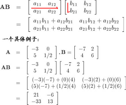
使用矩阵求解方程:
x ,y ,z = 2,1,5
x + y + z = 8
2x - y + z = 8
3x + y - z = 2
>>>X = np.array([[1,1,1],[2,-1,1], [3,1,-1]])

>>>X

array([[ 1,  1,  1],
       [ 2, -1,  1],
       [ 3,  1, -1]])

>>>Y = np.array([8,8,2])

>>>Y
array([8, 8, 2])

# W是我们要求解的未知数
>>>W = np.array(['x', 'y', 'z'])

>>>W
array(['x', 'y', 'z'], dtype='<U1')

# W = Y/X,但是在矩阵运算中没有除法,我们可以利用逆矩阵

# 求X的逆矩阵
>>>X_inv = np.linalg.inv(X)

>>>X_inv

array([[ 0. ,  0.2,  0.2],
       [ 0.5, -0.4,  0.1],
       [ 0.5,  0.2, -0.3]])

>>>W = np.dot(X_inv,Y)

>>>W
array([2., 1., 5.])
2、广播机制
【重要】ndarray广播机制的两条规则
- 规则一:为缺失的维度补1
- 规则二:假定缺失元素用已有值填充
>>>m = np.ones((2,3))

>>>m

array([[1., 1., 1.],
       [1., 1., 1.]])

>>>n = np.arange(3)

>>>n

array([0, 1, 2])

>>> m+n

array([[1., 2., 3.],
       [1., 2., 3.]])
七、ndarray的排序
1、快速排序
np.sort()与ndarray.sort()都可以,但是有区别:
np.sort()不改变输出
ndarray.sort()本地处理,不占用空间,单改变输出
2、部分排序
np.partition(a,k)
有的时候我们不是对全部数据感兴趣,我们可能只对最小或最大的一部分感兴趣。
- 当k为正时,我们想要得到最小的k个数
- 当k为负时,我们想要得到最大的k个数
>>>nd = np.random.randint(0,10000,size = 100)

>>>nd

array([2668, 3351,  780, 7451,  855, 9932, 2742, 3698, 2692, 7714,  325,
       9305, 9389, 8540, 2224, 1031, 9042, 5826, 3802, 9412, 1685, 9579,
       9828, 9943, 7272, 4380,  394, 5369,  803, 6454, 2250, 3377, 2660,
        522, 7149, 5752, 3309, 5143, 3914, 9850, 2657, 4221, 9730, 3073,
       6981, 2396, 5629, 3282, 7432, 1364, 5978,   98, 4110, 1782, 9996,
       3919,  162, 8594, 9344, 6253, 8339, 8287, 4015, 2927,  917, 1182,
       2286, 3454, 9525, 2566, 1253, 3988, 3209, 6287, 8175, 7825, 9815,
       1820, 9044, 9823, 5678, 6157,  465,  849, 9067, 1075, 1548, 3329,
         50, 6813,  281, 6275,  145, 7289, 7081,  911, 6118, 8315, 4973,
       8659])
>>>np.partition(nd,kth = 5)[:5]
array([ 50, 145,  98, 162, 281])

>>>np.partition(nd,kth = -5)[-5:]
array([9828, 9850, 9932, 9943, 9996])
八、练习题
1、创建一个长度为10的一维全为0的ndarray对象,然后让第五个元素等于1
>>>nd1 = np.zeros(shape=(10), dtype=np.int8)
>>>nd1[4]=1
>>>nd1

array([0, 0, 0, 0, 1, 0, 0, 0, 0, 0], dtype=int8)
2、创建一个元素从10到49的ndarray对象
>>>nd = np.arange(10,50,dtype=np.int8)
>>>nd

array([10, 11, 12, 13, 14, 15, 16, 17, 18, 19, 20, 21, 22, 23, 24, 25, 26,
       27, 28, 29, 30, 31, 32, 33, 34, 35, 36, 37, 38, 39, 40, 41, 42, 43,
       44, 45, 46, 47, 48, 49], dtype=int8)
>>>nd = np.array(range(10,49),dtype=np.int8)
>>>nd

array([10, 11, 12, 13, 14, 15, 16, 17, 18, 19, 20, 21, 22, 23, 24, 25, 26,
       27, 28, 29, 30, 31, 32, 33, 34, 35, 36, 37, 38, 39, 40, 41, 42, 43,
       44, 45, 46, 47, 48], dtype=int8)
3、将第二题反转
>>>nd[::-1]

array([48, 47, 46, 45, 44, 43, 42, 41, 40, 39, 38, 37, 36, 35, 34, 33, 32,
       31, 30, 29, 28, 27, 26, 25, 24, 23, 22, 21, 20, 19, 18, 17, 16, 15,
       14, 13, 12, 11, 10], dtype=int8)
4、使用np.random.random创建一个10*10的ndarray对象,并打印出最大最小元素
nd = np.random.random(size=(10,10))
print(np.max(nd), np.min(nd))
5、创建一个10*10的ndarray对象,且矩阵边界全为1,里面全为0
nd = np.ones(shape=(10,10))
nd[1:-1,1:-1]=0
nd
nd = np.zeros(shape=(10,10))
nd[[0,-1]]=1
nd[:,[0,-1]]=1
nd
6、创建一个每一行都是从0到4的5*5矩阵
nd = np.zeros(shape=(5,5))
nd1 = np.arange(5)
nd[:] = nd1
nd
nd = np.array([0,1,2,3,4]*5)
nd.reshape(5,5)
7、创建一个返回在(0,1)之间长度为12的等差数列
nd = np.linspace(0,1,12)
8、创建一个长度为10的随机数组并排序
nd = np.random.randint(0,100,size=(10))
nd.sort()
nd
9、创建一个长度为10的随机数组并将最大值替换为0
nd = np.random.randint(0,100,size=(10))
nd[np.argmax(nd)] = 0
10、如何根据第3列来对一个5*5矩阵排序?
nd = np.random.randint(0,100, size=(5,5))
sort_index = nd[:,2].argsort()
nd[sort_index]
11、给定一个4维矩阵,如何得到最后两维的和
nd = np.random.randint(0,10, size=(2,3,4,5))
nd1 = nd.sum(axis=(-1,-2))
nd1
nd1 = nd.sum(axis=-1).sum(axis=-1)
nd1
12、给定数组[1,2,3,4,5],如何得到在这个数组的每个元素之间插入3个0后的新数组
nd = np.array([1,2,3,4,5])
nd0 = np.zeros(17, dtype=np.int8)
nd0[::4]=nd
nd0
13、给定一个二维矩阵,如何交换其种两行的元素?
nd = np.random.randint(0,100, size=(2,3))
nd1 = np.vstack([nd[1],nd[0]])
nd = np.random.randint(0,100, size=(2,3))
nd[[1,0]]
14、创建一个100000长度的随机素
nd = np.random.randn(100000)
%%time
np.power(nd,3)
%%time
ret = []
for i in nd:
    ret.append(i**3)
15、创建一个5*3随机矩阵和一个3*2随机矩阵,求矩阵积
nd1 = np.random.randint(0,100, size=(5,3))
nd2 = np.random.randint(0,100, size=(3,2))
np.dot(nd1,nd2)
16、矩阵的每一行元素都减去改行的平均值
nd = np.random.randint(0,10, size=(4,5))
v_mean = nd.mean(axis=1)

nd-v_mean.reshape(4,1)
17、实现冒泡排序
nd = np.random.randint(0,100, size=20)
for i in range(20):
    for j in range(i,20):
        if nd[i] > nd[j]:
            nd[i],nd[j] = nd[j],nd[i]