原创文章,同步首发自作者个人博客 。转载请务必在文章开头显眼处注明出处
摘要
本文详述了如何通过数据预览,探索式数据分析,缺失数据填补,删除关联特征以及派生新特征等方法,在Kaggle的Titanic幸存预测这一分类问题竞赛中获得前2%排名的具体方法。
竞赛内容介绍
Titanic幸存预测是Kaggle上参赛人数最多的竞赛之一。它要求参赛选手通过训练数据集分析出什么类型的人更可能幸存,并预测出测试数据集中的所有乘客是否生还。
该项目是一个二元分类问题
如何取得排名前2%的成绩
加载数据
在加载数据之前,先通过如下代码加载之后会用到的所有R库
library(readr) # File read / write
library(ggplot2) # Data visualization
library(ggthemes) # Data visualization
library(scales) # Data visualization
library(plyr)
library(stringr) # String manipulation
library(InformationValue) # IV / WOE calculation
library(MLmetrics) # Mache learning metrics.e.g. Recall, Precision, Accuracy, AUC
library(rpart) # Decision tree utils
library(randomForest) # Random Forest
library(dplyr) # Data manipulation
library(e1071) # SVM
library(Amelia) # Missing value utils
library(party) # Conditional inference trees
library(gbm) # AdaBoost
library(class) # KNN
library(scales)
通过如下代码将训练数据和测试数据分别加载到名为train和test的data.frame中
train <- read_csv("train.csv")
test <- read_csv("test.csv")
由于之后需要对训练数据和测试数据做相同的转换,为避免重复操作和出现不一至的情况,更为了避免可能碰到的Categorical类型新level的问题,这里建议将训练数据和测试数据合并,统一操作。
data <- bind_rows(train, test)
train.row <- 1:nrow(train)
test.row <- (1 + nrow(train)):(nrow(train) + nrow(test))
数据预览
先观察数据
str(data)
## Classes 'tbl_df', 'tbl' and 'data.frame':    1309 obs. of  12 variables:
##  $ PassengerId: int  1 2 3 4 5 6 7 8 9 10 ...
##  $ Survived   : int  0 1 1 1 0 0 0 0 1 1 ...
##  $ Pclass     : int  3 1 3 1 3 3 1 3 3 2 ...
##  $ Name       : chr  "Braund, Mr. Owen Harris" "Cumings, Mrs. John Bradley (Florence Briggs Thayer)" "Heikkinen, Miss. Laina" "Futrelle, Mrs. Jacques Heath (Lily May Peel)" ...
##  $ Sex        : chr  "male" "female" "female" "female" ...
##  $ Age        : num  22 38 26 35 35 NA 54 2 27 14 ...
##  $ SibSp      : int  1 1 0 1 0 0 0 3 0 1 ...
##  $ Parch      : int  0 0 0 0 0 0 0 1 2 0 ...
##  $ Ticket     : chr  "A/5 21171" "PC 17599" "STON/O2. 3101282" "113803" ...
##  $ Fare       : num  7.25 71.28 7.92 53.1 8.05 ...
##  $ Cabin      : chr  NA "C85" NA "C123" ...
##  $ Embarked   : chr  "S" "C" "S" "S" ...
从上可见,数据集包含12个变量,1309条数据,其中891条为训练数据,418条为测试数据
- PassengerId 整型变量,标识乘客的ID,递增变量,对预测无帮助
- Survived 整型变量,标识该乘客是否幸存。0表示遇难,1表示幸存。将其转换为factor变量比较方便处理
- Pclass 整型变量,标识乘客的社会-经济状态,1代表Upper,2代表Middle,3代表Lower
- Name 字符型变量,除包含姓和名以外,还包含Mr. Mrs. Dr.这样的具有西方文化特点的信息
- Sex 字符型变量,标识乘客性别,适合转换为factor类型变量
- Age 整型变量,标识乘客年龄,有缺失值
- SibSp 整型变量,代表兄弟姐妹及配偶的个数。其中Sib代表Sibling也即兄弟姐妹,Sp代表Spouse也即配偶
- Parch 整型变量,代表父母或子女的个数。其中Par代表Parent也即父母,Ch代表Child也即子女
- Ticket 字符型变量,代表乘客的船票号
- Fare 数值型,代表乘客的船票价
- Cabin 字符型,代表乘客所在的舱位,有缺失值
- Embarked 字符型,代表乘客登船口岸,适合转换为factor型变量
探索式数据分析
乘客社会等级越高,幸存率越高
对于第一个变量Pclass,先将其转换为factor类型变量。
data$Survived <- factor(data$Survived)
可通过如下方式统计出每个Pclass幸存和遇难人数,如下
ggplot(data = data[1:nrow(train),], mapping = aes(x = Pclass, y = ..count.., fill=Survived)) +
  geom_bar(stat = "count", position='dodge') +
  xlab('Pclass') +
  ylab('Count') +
  ggtitle('How Pclass impact survivor') +
  scale_fill_manual(values=c("#FF0000", "#00FF00")) +
  geom_text(stat = "count", aes(label = ..count..), position=position_dodge(width=1), , vjust=-0.5) +
  theme(plot.title = element_text(hjust = 0.5), legend.position="bottom")
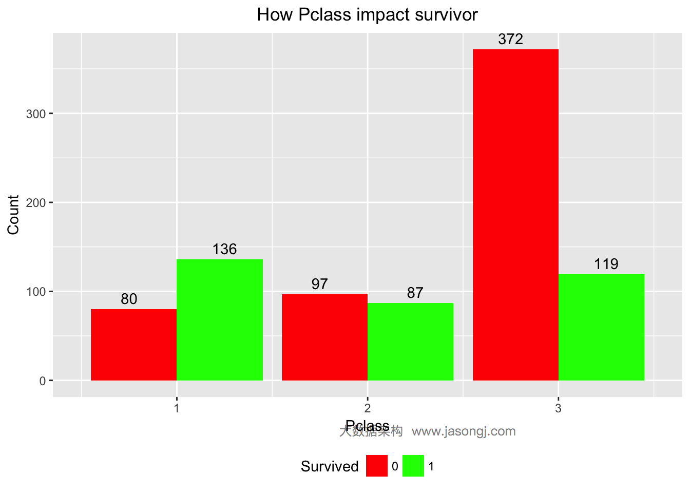
从上图可见,Pclass=1的乘客大部分幸存,Pclass=2的乘客接近一半幸存,而Pclass=3的乘客只有不到25%幸存。
为了更为定量的计算Pclass的预测价值,可以算出Pclass的WOE和IV如下。从结果可以看出,Pclass的IV为0.5,且“Highly Predictive”。由此可以暂时将Pclass作为预测模型的特征变量之一。
WOETable(X=factor(data$Pclass[1:nrow(train)]), Y=data$Survived[1:nrow(train)])
##   CAT GOODS BADS TOTAL     PCT_G     PCT_B        WOE         IV
## 1   1   136   80   216 0.3976608 0.1457195  1.0039160 0.25292792
## 2   2    87   97   184 0.2543860 0.1766849  0.3644848 0.02832087
## 3   3   119  372   491 0.3479532 0.6775956 -0.6664827 0.21970095
IV(X=factor(data$Pclass[1:nrow(train)]), Y=data$Survived[1:nrow(train)])
## [1] 0.5009497
## attr(,"howgood")
## [1] "Highly Predictive"
不同Title的乘客幸存率不同
乘客姓名重复度太低,不适合直接使用。而姓名中包含Mr. Mrs. Dr.等具有文化特征的信息,可将之抽取出来。
本文使用如下方式从姓名中抽取乘客的Title
data$Title <- sapply(data$Name, FUN=function(x) {strsplit(x, split='[,.]')[[1]][2]})
data$Title <- sub(' ', '', data$Title)
data$Title[data$Title %in% c('Mme', 'Mlle')] <- 'Mlle'
data$Title[data$Title %in% c('Capt', 'Don', 'Major', 'Sir')] <- 'Sir'
data$Title[data$Title %in% c('Dona', 'Lady', 'the Countess', 'Jonkheer')] <- 'Lady'
data$Title <- factor(data$Title)
抽取完乘客的Title后,统计出不同Title的乘客的幸存与遇难人数
ggplot(data = data[1:nrow(train),], mapping = aes(x = Title, y = ..count.., fill=Survived)) +
  geom_bar(stat = "count", position='stack') +
  xlab('Title') +
  ylab('Count') +
  ggtitle('How Title impact survivor') +
  scale_fill_discrete(name="Survived", breaks=c(0, 1), labels=c("Perish", "Survived")) +
  geom_text(stat = "count", aes(label = ..count..), position=position_stack(vjust = 0.5)) +
  theme(plot.title = element_text(hjust = 0.5), legend.position="bottom")
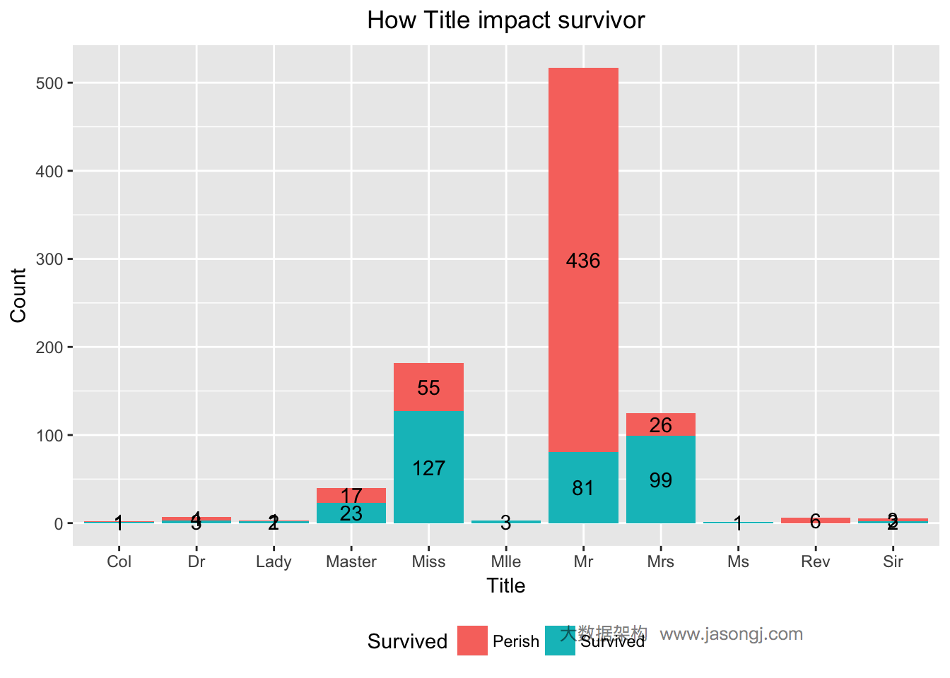
从上图可看出,Title为Mr的乘客幸存比例非常小,而Title为Mrs和Miss的乘客幸存比例非常大。这里使用WOE和IV来定量计算Title这一变量对于最终的预测是否有用。从计算结果可见,IV为1.520702,且"Highly Predictive"。因此,可暂将Title作为预测模型中的一个特征变量。
WOETable(X=data$Title[1:nrow(train)], Y=data$Survived[1:nrow(train)])
##       CAT GOODS BADS TOTAL       PCT_G       PCT_B         WOE            IV
## 1     Col     1    1     2 0.002873563 0.001808318  0.46315552  4.933741e-04
## 2      Dr     3    4     7 0.008620690 0.007233273  0.17547345  2.434548e-04
## 3    Lady     2    1     3 0.005747126 0.001808318  1.15630270  4.554455e-03
## 4  Master    23   17    40 0.066091954 0.030741410  0.76543639  2.705859e-02
## 5    Miss   127   55   182 0.364942529 0.099457505  1.30000942  3.451330e-01
## 6    Mlle     3    3     3 0.008620690 0.005424955  0.46315552  1.480122e-03
## 7      Mr    81  436   517 0.232758621 0.788426763 -1.22003757  6.779360e-01
## 8     Mrs    99   26   125 0.284482759 0.047016275  1.80017883  4.274821e-01
## 9      Ms     1    1     1 0.002873563 0.001808318  0.46315552  4.933741e-04
## 10    Rev     6    6     6 0.017241379 0.010849910  0.46315552  2.960244e-03
## 11    Sir     2    3     5 0.005747126 0.005424955  0.05769041  1.858622e-05
IV(X=data$Title[1:nrow(train)], Y=data$Survived[1:nrow(train)])
## [1] 1.487853
## attr(,"howgood")
## [1] "Highly Predictive"
女性幸存率远高于男性
对于Sex变量,由Titanic号沉没的背景可知,逃生时遵循“妇女与小孩先走”的规则,由此猜想,Sex变量应该对预测乘客幸存有帮助。
如下数据验证了这一猜想,大部分女性(233/(233+81)=74.20%)得以幸存,而男性中只有很小部分(109/(109+468)=22.85%)幸存。
data$Sex <- as.factor(data$Sex)
ggplot(data = data[1:nrow(train),], mapping = aes(x = Sex, y = ..count.., fill=Survived)) +
  geom_bar(stat = 'count', position='dodge') +
  xlab('Sex') +
  ylab('Count') +
  ggtitle('How Sex impact survivo') +
  geom_text(stat = "count", aes(label = ..count..), position=position_dodge(width=1), , vjust=-0.5) +
  theme(plot.title = element_text(hjust = 0.5), legend.position="bottom")
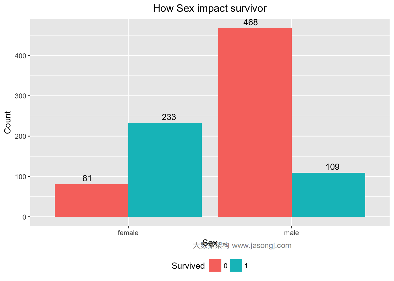
通过计算WOE和IV可知,Sex的IV为1.34且"Highly Predictive",可暂将Sex作为特征变量。
WOETable(X=data$Sex[1:nrow(train)], Y=data$Survived[1:nrow(train)])
##      CAT GOODS BADS TOTAL     PCT_G    PCT_B        WOE        IV
## 1 female   233   81   314 0.6812865 0.147541  1.5298770 0.8165651
## 2   male   109  468   577 0.3187135 0.852459 -0.9838327 0.5251163
IV(X=data$Sex[1:nrow(train)], Y=data$Survived[1:nrow(train)])
## [1] 1.341681
## attr(,"howgood")
## [1] "Highly Predictive"
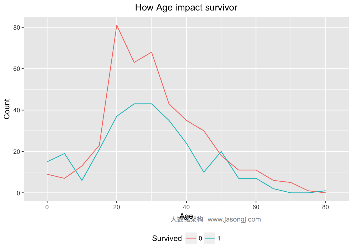
未成年人幸存率高于成年人
结合背景,按照“妇女与小孩先走”的规则,未成年人应该有更大可能幸存。如下图所示,Age < 18的乘客中,幸存人数确实高于遇难人数。同时青壮年乘客中,遇难人数远高于幸存人数。
ggplot(data = data[(!is.na(data$Age)) & row(data[, 'Age']) <= 891, ], aes(x = Age, color=Survived)) +
  geom_line(aes(label=..count..), stat = 'bin', binwidth=5)  +
  labs(title = "How Age impact survivor", x = "Age", y = "Count", fill = "Survived")
## Warning: Ignoring unknown aesthetics: label
配偶及兄弟姐妹数适中的乘客更易幸存
对于SibSp变量,分别统计出幸存与遇难人数。
ggplot(data = data[1:nrow(train),], mapping = aes(x = SibSp, y = ..count.., fill=Survived)) +
  geom_bar(stat = 'count', position='dodge') +
  labs(title = "How SibSp impact survivor", x = "Sibsp", y = "Count", fill = "Survived") +
  geom_text(stat = "count", aes(label = ..count..), position=position_dodge(width=1), , vjust=-0.5) +
  theme(plot.title = element_text(hjust = 0.5), legend.position="bottom")
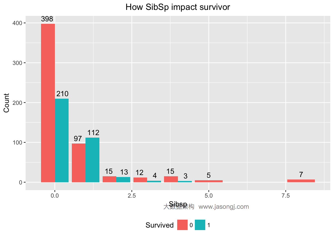
从上图可见,SibSp为0的乘客,幸存率低于1/3;SibSp为1或2的乘客,幸存率高于50%;SibSp大于等于3的乘客,幸存率非常低。可通过计算WOE与IV定量计算SibSp对预测的贡献。IV为0.1448994,且"Highly Predictive"。
WOETable(X=as.factor(data$SibSp[1:nrow(train)]), Y=data$Survived[1:nrow(train)])
##   CAT GOODS BADS TOTAL       PCT_G       PCT_B        WOE          IV
## 1   0   210  398   608 0.593220339 0.724954463 -0.2005429 0.026418349
## 2   1   112   97   209 0.316384181 0.176684882  0.5825894 0.081387334
## 3   2    13   15    28 0.036723164 0.027322404  0.2957007 0.002779811
## 4   3     4   12    16 0.011299435 0.021857923 -0.6598108 0.006966604
## 5   4     3   15    18 0.008474576 0.027322404 -1.1706364 0.022063953
## 6   5     5    5     5 0.014124294 0.009107468  0.4388015 0.002201391
## 7   8     7    7     7 0.019774011 0.012750455  0.4388015 0.003081947
IV(X=as.factor(data$SibSp[1:nrow(train)]), Y=data$Survived[1:nrow(train)])
## [1] 0.1448994
## attr(,"howgood")
## [1] "Highly Predictive"
父母与子女数为1到3的乘客更可能幸存
对于Parch变量,分别统计出幸存与遇难人数。
ggplot(data = data[1:nrow(train),], mapping = aes(x = Parch, y = ..count.., fill=Survived)) +
  geom_bar(stat = 'count', position='dodge') +
  labs(title = "How Parch impact survivor", x = "Parch", y = "Count", fill = "Survived") +
  geom_text(stat = "count", aes(label = ..count..), position=position_dodge(width=1), , vjust=-0.5) +
  theme(plot.title = element_text(hjust = 0.5), legend.position="bottom")
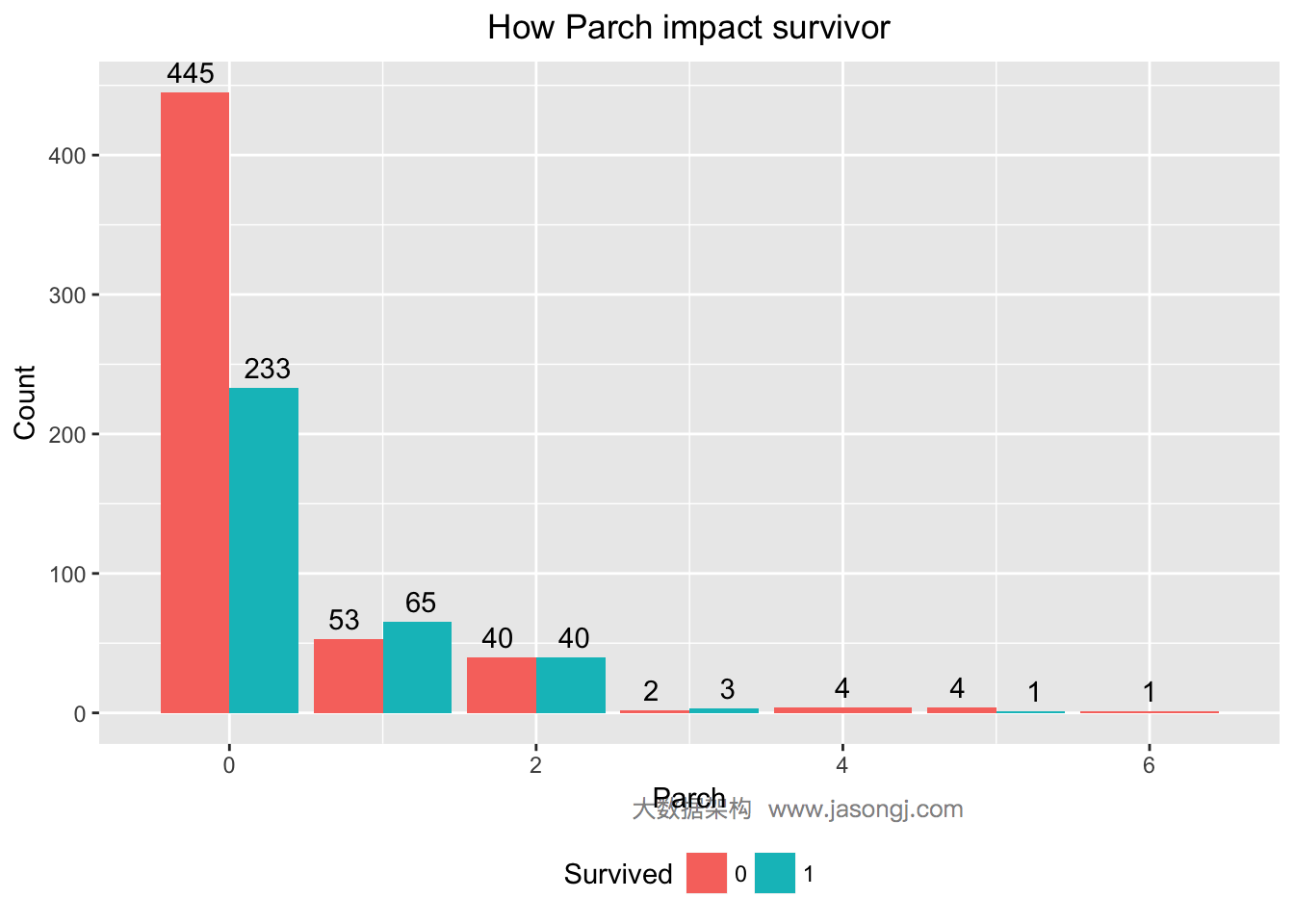
从上图可见,Parch为0的乘客,幸存率低于1/3;Parch为1到3的乘客,幸存率高于50%;Parch大于等于4的乘客,幸存率非常低。可通过计算WOE与IV定量计算Parch对预测的贡献。IV为0.1166611,且"Highly Predictive"。
WOETable(X=as.factor(data$Parch[1:nrow(train)]), Y=data$Survived[1:nrow(train)])
##   CAT GOODS BADS TOTAL       PCT_G       PCT_B        WOE          IV
## 1   0   233  445   678 0.671469741 0.810564663 -0.1882622 0.026186312
## 2   1    65   53   118 0.187319885 0.096539162  0.6628690 0.060175728
## 3   2    40   40    80 0.115273775 0.072859745  0.4587737 0.019458440
## 4   3     3    2     5 0.008645533 0.003642987  0.8642388 0.004323394
## 5   4     4    4     4 0.011527378 0.007285974  0.4587737 0.001945844
## 6   5     1    4     5 0.002881844 0.007285974 -0.9275207 0.004084922
## 7   6     1    1     1 0.002881844 0.001821494  0.4587737 0.000486461
IV(X=as.factor(data$Parch[1:nrow(train)]), Y=data$Survived[1:nrow(train)])
## [1] 0.1166611
## attr(,"howgood")
## [1] "Highly Predictive"
FamilySize为2到4的乘客幸存可能性较高
SibSp与Parch都说明,当乘客无亲人时,幸存率较低,乘客有少数亲人时,幸存率高于50%,而当亲人数过高时,幸存率反而降低。在这里,可以考虑将SibSp与Parch相加,生成新的变量,FamilySize。
data$FamilySize <- data$SibSp + data$Parch + 1
ggplot(data = data[1:nrow(train),], mapping = aes(x = FamilySize, y = ..count.., fill=Survived)) +
  geom_bar(stat = 'count', position='dodge') +
  xlab('FamilySize') +
  ylab('Count') +
  ggtitle('How FamilySize impact survivor') +
  geom_text(stat = "count", aes(label = ..count..), position=position_dodge(width=1), , vjust=-0.5) +
  theme(plot.title = element_text(hjust = 0.5), legend.position="bottom")
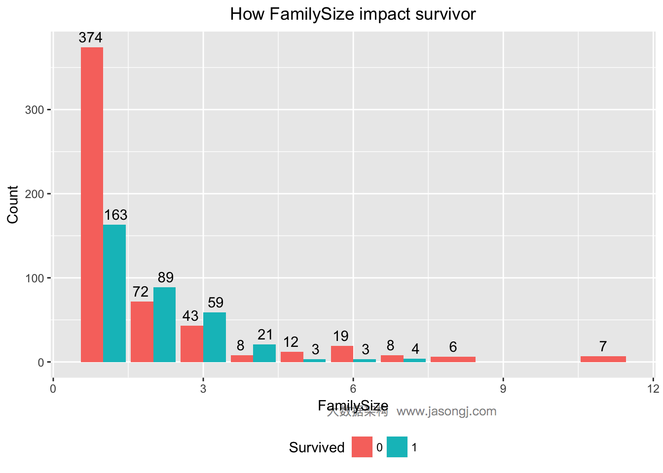
计算FamilySize的WOE和IV可知,IV为0.3497672,且“Highly Predictive”。由SibSp与Parch派生出来的新变量FamilySize的IV高于SibSp与Parch的IV,因此,可将这个派生变量FamilySize作为特征变量。
WOETable(X=as.factor(data$FamilySize[1:nrow(train)]), Y=data$Survived[1:nrow(train)])
##   CAT GOODS BADS TOTAL       PCT_G      PCT_B        WOE           IV
## 1   1   163  374   537 0.459154930 0.68123862 -0.3945249 0.0876175539
## 2   2    89   72   161 0.250704225 0.13114754  0.6479509 0.0774668616
## 3   3    59   43   102 0.166197183 0.07832423  0.7523180 0.0661084057
## 4   4    21    8    29 0.059154930 0.01457195  1.4010615 0.0624634998
## 5   5     3   12    15 0.008450704 0.02185792 -0.9503137 0.0127410643
## 6   6     3   19    22 0.008450704 0.03460838 -1.4098460 0.0368782940
## 7   7     4    8    12 0.011267606 0.01457195 -0.2571665 0.0008497665
## 8   8     6    6     6 0.016901408 0.01092896  0.4359807 0.0026038712
## 9  11     7    7     7 0.019718310 0.01275046  0.4359807 0.0030378497
IV(X=as.factor(data$FamilySize[1:nrow(train)]), Y=data$Survived[1:nrow(train)])
## [1] 0.3497672
## attr(,"howgood")
## [1] "Highly Predictive"
共票号乘客幸存率高
对于Ticket变量,重复度非常低,无法直接利用。先统计出每张票对应的乘客数。
ticket.count <- aggregate(data$Ticket, by = list(data$Ticket), function(x) sum(!is.na(x)))
这里有个猜想,票号相同的乘客,是一家人,很可能同时幸存或者同时遇难。现将所有乘客按照Ticket分为两组,一组是使用单独票号,另一组是与他人共享票号,并统计出各组的幸存与遇难人数。
data$TicketCount <- apply(data, 1, function(x) ticket.count[which(ticket.count[, 1] == x['Ticket']), 2])
data$TicketCount <- factor(sapply(data$TicketCount, function(x) ifelse(x > 1, 'Share', 'Unique')))
ggplot(data = data[1:nrow(train),], mapping = aes(x = TicketCount, y = ..count.., fill=Survived)) +
  geom_bar(stat = 'count', position='dodge') +
  xlab('TicketCount') +
  ylab('Count') +
  ggtitle('How TicketCount impact survivor') +
  geom_text(stat = "count", aes(label = ..count..), position=position_dodge(width=1), , vjust=-0.5) +
  theme(plot.title = element_text(hjust = 0.5), legend.position="bottom")
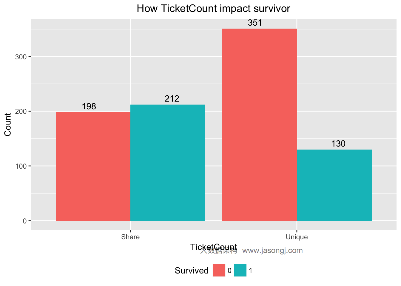
由上图可见,未与他人同票号的乘客,只有130/(130+351)=27%幸存,而与他人同票号的乘客有212/(212+198)=51.7%幸存。计算TicketCount的WOE与IV如下。其IV为0.2751882,且"Highly Predictive"
WOETable(X=data$TicketCount[1:nrow(train)], Y=data$Survived[1:nrow(train)])
##      CAT GOODS BADS TOTAL    PCT_G     PCT_B        WOE        IV
## 1  Share   212  198   410 0.619883 0.3606557  0.5416069 0.1403993
## 2 Unique   130  351   481 0.380117 0.6393443 -0.5199641 0.1347889
IV(X=data$TicketCount[1:nrow(train)], Y=data$Survived[1:nrow(train)])
## [1] 0.2751882
## attr(,"howgood")
## [1] "Highly Predictive"
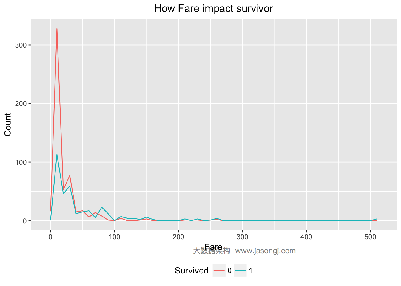
支出船票费越高幸存率越高
对于Fare变量,由下图可知,Fare越大,幸存率越高。
ggplot(data = data[(!is.na(data$Fare)) & row(data[, 'Fare']) <= 891, ], aes(x = Fare, color=Survived)) +
  geom_line(aes(label=..count..), stat = 'bin', binwidth=10)  +
  labs(title = "How Fare impact survivor", x = "Fare", y = "Count", fill = "Survived")
不同仓位的乘客幸存率不同
对于Cabin变量,其值以字母开始,后面伴以数字。这里有一个猜想,字母代表某个区域,数据代表该区域的序号。类似于火车票即有车箱号又有座位号。因此,这里可尝试将Cabin的首字母提取出来,并分别统计出不同首字母仓位对应的乘客的幸存率。
ggplot(data[1:nrow(train), ], mapping = aes(x = as.factor(sapply(data$Cabin[1:nrow(train)], function(x) str_sub(x, start = 1, end = 1))), y = ..count.., fill = Survived)) +
  geom_bar(stat = 'count', position='dodge') +
  xlab('Cabin') +
  ylab('Count') +
  ggtitle('How Cabin impact survivor') +
  geom_text(stat = "count", aes(label = ..count..), position=position_dodge(width=1), , vjust=-0.5) +
  theme(plot.title = element_text(hjust = 0.5), legend.position="bottom")
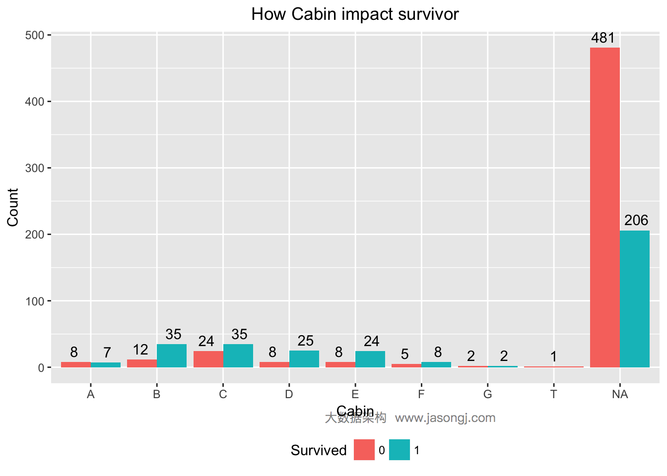
由上图可见,仓位号首字母为B,C,D,E,F的乘客幸存率均高于50%,而其它仓位的乘客幸存率均远低于50%。仓位变量的WOE及IV计算如下。由此可见,Cabin的IV为0.1866526,且“Highly Predictive”
data$Cabin <- sapply(data$Cabin, function(x) str_sub(x, start = 1, end = 1))
WOETable(X=as.factor(data$Cabin[1:nrow(train)]), Y=data$Survived[1:nrow(train)])
##   CAT GOODS BADS TOTAL      PCT_G      PCT_B        WOE          IV
## 1   A     7    8    15 0.05109489 0.11764706 -0.8340046 0.055504815
## 2   B    35   12    47 0.25547445 0.17647059  0.3699682 0.029228917
## 3   C    35   24    59 0.25547445 0.35294118 -0.3231790 0.031499197
## 4   D    25    8    33 0.18248175 0.11764706  0.4389611 0.028459906
## 5   E    24    8    32 0.17518248 0.11764706  0.3981391 0.022907100
## 6   F     8    5    13 0.05839416 0.07352941 -0.2304696 0.003488215
## 7   G     2    2     4 0.01459854 0.02941176 -0.7004732 0.010376267
## 8   T     1    1     1 0.00729927 0.01470588 -0.7004732 0.005188134
IV(X=as.factor(data$Cabin[1:nrow(train)]), Y=data$Survived[1:nrow(train)])
## [1] 0.1866526
## attr(,"howgood")
## [1] "Highly Predictive"
Embarked为S的乘客幸存率较低
Embarked变量代表登船码头,现通过统计不同码头登船的乘客幸存率来判断Embarked是否可用于预测乘客幸存情况。
ggplot(data[1:nrow(train), ], mapping = aes(x = Embarked, y = ..count.., fill = Survived)) +
  geom_bar(stat = 'count', position='dodge') +
  xlab('Embarked') +
  ylab('Count') +
  ggtitle('How Embarked impact survivor') +
  geom_text(stat = "count", aes(label = ..count..), position=position_dodge(width=1), , vjust=-0.5) +
  theme(plot.title = element_text(hjust = 0.5), legend.position="bottom")
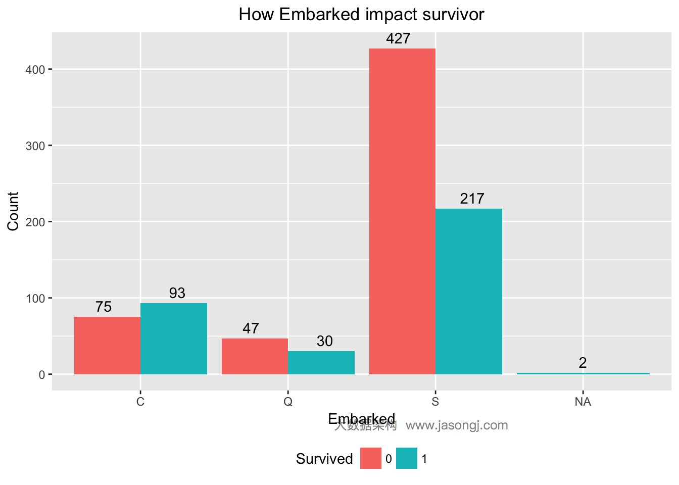
从上图可见,Embarked为S的乘客幸存率仅为217/(217+427)=33.7%,而Embarked为C或为NA的乘客幸存率均高于50%。初步判断Embarked可用于预测乘客是否幸存。Embarked的WOE和IV计算如下。
WOETable(X=as.factor(data$Embarked[1:nrow(train)]), Y=data$Survived[1:nrow(train)])
##   CAT GOODS BADS TOTAL      PCT_G     PCT_B        WOE           IV
## 1   C    93   75   168 0.27352941 0.1366120  0.6942642 9.505684e-02
## 2   Q    30   47    77 0.08823529 0.0856102  0.0302026 7.928467e-05
## 3   S   217  427   644 0.63823529 0.7777778 -0.1977338 2.759227e-02
IV(X=as.factor(data$Embarked[1:nrow(train)]), Y=data$Survived[1:nrow(train)])
## [1] 0.1227284
## attr(,"howgood")
## [1] "Highly Predictive"
从上述计算结果可见,IV为0.1227284,且“Highly Predictive”。
填补缺失值
列出所有缺失数据
attach(data)
  missing <- list(Pclass=nrow(data[is.na(Pclass), ]))
  missing$Name <- nrow(data[is.na(Name), ])
  missing$Sex <- nrow(data[is.na(Sex), ])
  missing$Age <- nrow(data[is.na(Age), ])
  missing$SibSp <- nrow(data[is.na(SibSp), ])
  missing$Parch <- nrow(data[is.na(Parch), ])
  missing$Ticket <- nrow(data[is.na(Ticket), ])
  missing$Fare <- nrow(data[is.na(Fare), ])
  missing$Cabin <- nrow(data[is.na(Cabin), ])
  missing$Embarked <- nrow(data[is.na(Embarked), ])
  for (name in names(missing)) {
    if (missing[[name]][1] > 0) {
      print(paste('', name, ' miss ', missing[[name]][1], ' values', sep = ''))
    }
  }
detach(data)
## [1] "Age miss 263 values"
## [1] "Fare miss 1 values"
## [1] "Cabin miss 1014 values"
## [1] "Embarked miss 2 values"
预测乘客年龄
缺失年龄信息的乘客数为263,缺失量比较大,不适合使用中位数或者平均值填补。一般通过使用其它变量预测或者直接将缺失值设置为默认值的方法填补,这里通过其它变量来预测缺失的年龄信息。
age.model <- rpart(Age ~ Pclass + Sex + SibSp + Parch + Fare + Embarked + Title + FamilySize, data=data[!is.na(data$Age), ], method='anova')
data$Age[is.na(data$Age)] <- predict(age.model, data[is.na(data$Age), ])
中位数填补缺失的Embarked值
从如下数据可见,缺失Embarked信息的乘客的Pclass均为1,且Fare均为80。
data[is.na(data$Embarked), c('PassengerId', 'Pclass', 'Fare', 'Embarked')]
## # A tibble: 2 × 4
##   PassengerId Pclass  Fare Embarked
##         <int>  <int> <dbl>    <chr>
## 1          62      1    80     <NA>
## 2         830      1    80     <NA>
由下图所见,Embarked为C且Pclass为1的乘客的Fare中位数为80。
ggplot(data[!is.na(data$Embarked),], aes(x=Embarked, y=Fare, fill=factor(Pclass))) +
  geom_boxplot() +
  geom_hline(aes(yintercept=80), color='red', linetype='dashed', lwd=2) +
  scale_y_continuous(labels=dollar_format()) + theme_few()
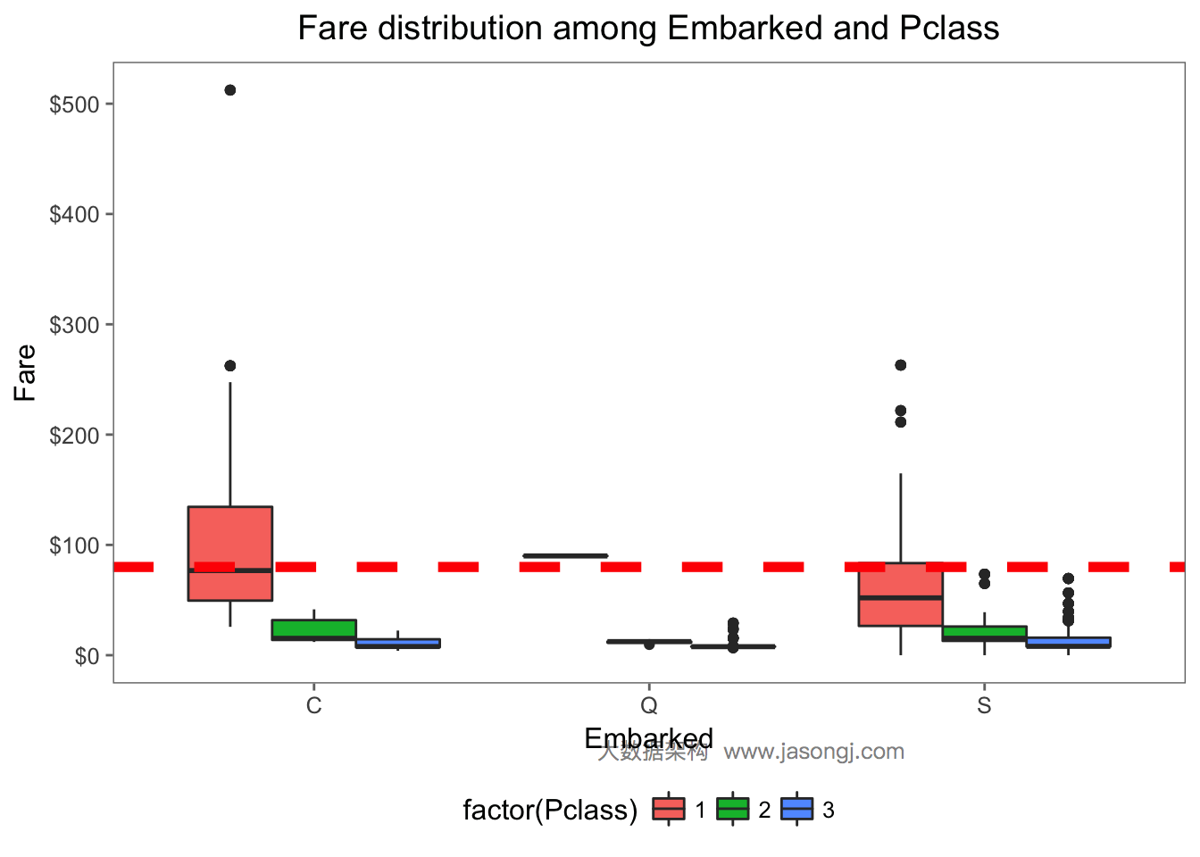
因此可以将缺失的Embarked值设置为'C'。
data$Embarked[is.na(data$Embarked)] <- 'C'
data$Embarked <- as.factor(data$Embarked)
中位数填补一个缺失的Fare值
由于缺失Fare值的记录非常少,一般可直接使用平均值或者中位数填补该缺失值。这里使用乘客的Fare中位数填补缺失值。
data$Fare[is.na(data$Fare)] <- median(data$Fare, na.rm=TRUE)
将缺失的Cabin设置为默认值
缺失Cabin信息的记录数较多,不适合使用中位数或者平均值填补,一般通过使用其它变量预测或者直接将缺失值设置为默认值的方法填补。由于Cabin信息不太容易从其它变量预测,并且在上一节中,将NA单独对待时,其IV已经比较高。因此这里直接将缺失的Cabin设置为一个默认值。
data$Cabin <- as.factor(sapply(data$Cabin, function(x) ifelse(is.na(x), 'X', str_sub(x, start = 1, end = 1))))
训练模型
set.seed(415)
model <- cforest(Survived ~ Pclass + Title + Sex + Age + SibSp + Parch + FamilySize + TicketCount + Fare + Cabin + Embarked, data = data[train.row, ], controls=cforest_unbiased(ntree=2000, mtry=3))
交叉验证
一般情况下,应该将训练数据分为两部分,一部分用于训练,另一部分用于验证。或者使用k-fold交叉验证。本文将所有训练数据都用于训练,然后随机选取30%数据集用于验证。
cv.summarize <- function(data.true, data.predict) {
  print(paste('Recall:', Recall(data.true, data.predict)))
  print(paste('Precision:', Precision(data.true, data.predict)))
  print(paste('Accuracy:', Accuracy(data.predict, data.true)))
  print(paste('AUC:', AUC(data.predict, data.true)))
}
set.seed(415)
cv.test.sample <- sample(1:nrow(train), as.integer(0.3 * nrow(train)), replace = TRUE)
cv.test <- data[cv.test.sample,]
cv.prediction <- predict(model, cv.test, OOB=TRUE, type = "response")
cv.summarize(cv.test$Survived, cv.prediction)
## [1] "Recall: 0.947976878612717"
## [1] "Precision: 0.841025641025641"
## [1] "Accuracy: 0.850187265917603"
## [1] "AUC: 0.809094822285082"
预测
predict.result <- predict(model, data[(1+nrow(train)):(nrow(data)), ], OOB=TRUE, type = "response")
output <- data.frame(PassengerId = test$PassengerId, Survived = predict.result)
write.csv(output, file = "cit1.csv", row.names = FALSE)
该模型预测结果在Kaggle的得分为0.80383,排第992名,前992/6292=15.8%。
调优
去掉关联特征
由于FamilySize结合了SibSp与Parch的信息,因此可以尝试将SibSp与Parch从特征变量中移除。
set.seed(415)
model <- cforest(Survived ~ Pclass + Title + Sex + Age + FamilySize + TicketCount + Fare + Cabin + Embarked, data = data[train.row, ], controls=cforest_unbiased(ntree=2000, mtry=3))
predict.result <- predict(model, data[test.row, ], OOB=TRUE, type = "response")
submit <- data.frame(PassengerId = test$PassengerId, Survived = predict.result)
write.csv(submit, file = "cit2.csv", row.names = FALSE)
该模型预测结果在Kaggle的得分仍为0.80383。
去掉IV较低的Cabin
由于Cabin的IV值相对较低,因此可以考虑将其从模型中移除。
set.seed(415)
model <- cforest(Survived ~ Pclass + Title + Sex + Age + FamilySize + TicketCount + Fare + Embarked, data = data[train.row, ], controls=cforest_unbiased(ntree=2000, mtry=3))
predict.result <- predict(model, data[test.row, ], OOB=TRUE, type = "response")
submit <- data.frame(PassengerId = test$PassengerId, Survived = predict.result)
write.csv(submit, file = "cit3.csv", row.names = FALSE)
该模型预测结果在Kaggle的得分仍为0.80383。
增加派生特征
对于Name变量,上文从中派生出了Title变量。由于以下原因,可推测乘客的姓氏可能具有一定的预测作用
- 部分西方国家中人名的重复度较高,而姓氏重复度较低,姓氏具有一定辨识度
- 部分国家的姓氏具有一定的身份识别作用
- 姓氏相同的乘客,可能是一家人(这一点也基于西方国家姓氏重复度较低这一特点),而一家人同时幸存或遇难的可能性较高
考虑到只出现一次的姓氏不可能同时出现在训练集和测试集中,不具辨识度和预测作用,因此将只出现一次的姓氏均命名为'Small'
data$Surname <- sapply(data$Name, FUN=function(x) {strsplit(x, split='[,.]')[[1]][1]})
data$FamilyID <- paste(as.character(data$FamilySize), data$Surname, sep="")
data$FamilyID[data$FamilySize <= 2] <- 'Small'
# Delete erroneous family IDs
famIDs <- data.frame(table(data$FamilyID))
famIDs <- famIDs[famIDs$Freq <= 2,]
data$FamilyID[data$FamilyID %in% famIDs$Var1] <- 'Small'
# Convert to a factor
data$FamilyID <- factor(data$FamilyID)
set.seed(415)
model <- cforest(as.factor(Survived) ~ Pclass + Sex + Age + Fare + Embarked + Title + FamilySize + FamilyID + TicketCount, data = data[train.row, ], controls=cforest_unbiased(ntree=2000, mtry=3))
predict.result <- predict(model, data[test.row, ], OOB=TRUE, type = "response")
submit <- data.frame(PassengerId = test$PassengerId, Survived = predict.result)
write.csv(submit, file = "cit4.csv", row.names = FALSE)
该模型预测结果在Kaggle的得分为0.82297,排第207名,前207/6292=3.3%
其它
经试验,将缺失的Embarked补充为出现最多的S而非C,成绩有所提升。但该方法理论依据不强,并且该成绩只是Public排行榜成绩,并非最终成绩,并不能说明该方法一定优于其它方法。因此本文并不推荐该方法,只是作为一种可能的思路,供大家参考学习。
data$Embarked[c(62,830)] = "S"
data$Embarked <- factor(data$Embarked)
set.seed(415)
model <- cforest(as.factor(Survived) ~ Pclass + Sex + Age + Fare + Embarked + Title + FamilySize + FamilyID + TicketCount, data = data[train.row, ], controls=cforest_unbiased(ntree=2000, mtry=3))
predict.result <- predict(model, data[test.row, ], OOB=TRUE, type = "response")
submit <- data.frame(PassengerId = test$PassengerId, Survived = predict.result)
write.csv(submit, file = "cit5.csv", row.names = FALSE)
该模型预测结果在Kaggle的得分仍为0.82775,排第114名,前114/6292=1.8%
![]()
总结
本文详述了如何通过数据预览,探索式数据分析,缺失数据填补,删除关联特征以及派生新特征等方法,在Kaggle的Titanic幸存预测这一分类问题竞赛中获得前2%排名的具体方法。
下篇预告
下一篇文章将侧重讲解使用机器学习解决工程问题的一般思路和方法。