R 《回归分析与线性统计模型》page141,5.2

rm(list = ls())
library(car)
library(MASS)
library(openxlsx)
A = read.xlsx("data141.xlsx")
head(A)

　　

fm = lm(y~x1+x2+x3+x4 , data=A )
#判断多重共线性
vif(fm)

　　

> vif(fm)
       x1        x2        x3        x4 
 38.49621 254.42317  46.86839 282.51286 #具有多重共线性

　　

#进行主成分回归
A.pr = princomp(~x1+x2+x3+x4 , data = A,cor=T)
summary(A.pr,loadings = T) #输出特征值和特征向量

　　

> summary(A.pr,loadings = T) #输出特征值和特征向量
Importance of components:
                         Comp.1    Comp.2     Comp.3       Comp.4
Standard deviation     1.495227 1.2554147 0.43197934 0.0402957285
Proportion of Variance 0.558926 0.3940165 0.04665154 0.0004059364
Cumulative Proportion  0.558926 0.9529425 0.99959406 1.0000000000

Loadings:
   Comp.1 Comp.2 Comp.3 Comp.4
x1  0.476  0.509  0.676  0.241
x2  0.564 -0.414 -0.314  0.642
x3 -0.394 -0.605  0.638  0.268
x4 -0.548  0.451 -0.195  0.677

　　

pre = predict(A.pr)  #主成分，组合向量，无实际意义
A$z1 = pre[,1]
A$z2 = pre[,2]       #根据累积贡献率，根据保留两个主成分变量

　　

lm.sol = lm(y~z1 + z2,data = A) #与主成分预测变量线性回归
lm.sol

> lm.sol

Call:
lm(formula = y ~ z1 + z2, data = A)

Coefficients:
(Intercept)           z1           z2  
    95.4231       9.4954      -0.1201  

> summary(lm.sol)      #模型详细

Call:
lm(formula = y ~ z1 + z2, data = A)

Residuals:
    Min      1Q  Median      3Q     Max 
-3.3305 -2.1882 -0.9491  1.0998  4.4251 

Coefficients:
            Estimate Std. Error t value Pr(>|t|)    
(Intercept)  95.4231     0.8548 111.635  < 2e-16 ***
z1            9.4954     0.5717  16.610 1.31e-08 ***
z2           -0.1201     0.6809  -0.176    0.864    
---
Signif. codes:  0 ‘***’ 0.001 ‘**’ 0.01 ‘*’ 0.05 ‘.’ 0.1 ‘ ’ 1

Residual standard error: 3.082 on 10 degrees of freedom
Multiple R-squared:  0.965,	Adjusted R-squared:  0.958 
F-statistic:   138 on 2 and 10 DF,  p-value: 5.233e-08

　　

beta = coef(lm.sol)  #主成分分析的预测变量的系数
beta

> beta
(Intercept)          z1          z2 
 95.4230769   9.4953702  -0.1200892 

　　

#预测变量还原
eigen_vec = loadings(A.pr) #特征向量
x.bar =  A.pr$center #均值？
x.sd = A.pr$scale    #标准误？
xishu_1 = (beta[2]*eigen_vec[,1])/x.sd
xishu_2 = (beta[3]*eigen_vec[,2])/x.sd
coef = xishu_1 + xishu_2
coef
beta0 = beta[1] - sum(x.bar*coef)
B = c(beta0,coef)
B #还原后的回归系数

　　

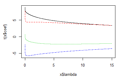
#岭估计
esti_ling = lm.ridge(y~x1+x2+x3+x4 , data = A, lambda = seq(0,15,0.01))
plot(esti_ling)

　　

#取k=5
k = 5
X = cbind(1,as.matrix(A[,2:5]))
y = A[,6]
B_ = solve((t(X)%*%X) + k*diag(5))%*%t(X)%*%y
B_

　　

> B_
         [,1]
   0.06158362
x1 2.12614307
x2 1.16796919
x3 0.71043177
x4 0.49566883