用R语言的quantreg包进行分位数回归

什么是分位数回归

分位数回归(Quantile Regression)是计量经济学的研究前沿方向之一，它利用解释变量的多个分位数（例如四分位、十分位、百分位等）来得到被解释变量的条件分布的相应的分位数方程。

与传统的OLS只得到均值方程相比，分位数回归可以更详细地描述变量的统计分布。它是给定回归变量X，估计响应变量Y条件分位数的一个基本方法；它不仅可以度量回归变量在分布中心的影响,而且还可以度量在分布上尾和下尾的影响，因此较之经典的最小二乘回归具有独特的优势。众所周知，经典的最小二乘回归是针对因变量的均值（期望）的：模型反映了因变量的均值怎样受自变量的影响，

y=βX+ϵy=βX+ϵ，E(y)=βXE(y)=βX

分位数回归的核心思想就是从均值推广到分位数。最小二乘回归的目标是最小化误差平方和，分位数回归也是最小化一个新的目标函数：

minξ∈R∑ρτ(yi−ξ)minξ∈R∑ρτ(yi−ξ)

quantreg包

quantreg即：Quantile Regression，拥有条件分位数模型的估计和推断方法，包括线性、非线性和非参模型；处理单变量响应的条件分位数方法；处理删失数据的几种方法。此外，还包括基于预期风险损失的投资组合选择方法。

实例

library(quantreg)  # 载入quantreg包
data(engel)        # 加载quantreg包自带的数据集

分位数回归(tau = 0.5)
fit1 = rq(foodexp ~ income, tau = 0.5, data = engel)         
r1 = resid(fit1)   # 得到残差序列，并赋值为变量r1
c1 = coef(fit1)    # 得到模型的系数，并赋值给变量c1

summary(fit1)      # 显示分位数回归的模型和系数
`
Call: rq(formula = foodexp ~ income, tau = 0.5, data = engel)

tau: [1] 0.5

Coefficients:
            coefficients lower bd  upper bd 
(Intercept)  81.48225     53.25915 114.01156
income        0.56018      0.48702   0.60199
`

summary(fit1, se = "boot") # 通过设置参数se，可以得到系数的假设检验
`
Call: rq(formula = foodexp ~ income, tau = 0.5, data = engel)

tau: [1] 0.5

Coefficients:
            Value    Std. Error t value  Pr(>|t|)
(Intercept) 81.48225 27.57092    2.95537  0.00344
income       0.56018  0.03507   15.97392  0.00000
`

分位数回归(tau = 0.5、0.75)
fit1 = rq(foodexp ~ income, tau = 0.5, data = engel) 
fit2 = rq(foodexp ~ income, tau = 0.75, data = engel)

模型比较
anova(fit1,fit2)    #方差分析
`   
Quantile Regression Analysis of Deviance Table

Model: foodexp ~ income
Joint Test of Equality of Slopes: tau in {  0.5 0.75  }

  Df Resid Df F value    Pr(>F)    
1  1      469  12.093 0.0005532 ***
---
Signif. codes:  0 ‘***’ 0.001 ‘**’ 0.01 ‘*’ 0.05 ‘.’ 0.1 ‘ ’ 1
`   
画图比较分析
plot(engel$foodexp , engel$income,pch=20, col = "#2E8B57",
     main = "家庭收入与食品支出的分位数回归",xlab="食品支出",ylab="家庭收入")
lines(fitted(fit1), engel$income,lwd=2, col = "#EEEE00")
lines(fitted(fit2), engel$income,lwd=2, col = "#EE6363")
legend("topright", c("tau=.5","tau=.75"), lty=c(1,1),
       col=c("#EEEE00","#EE6363"))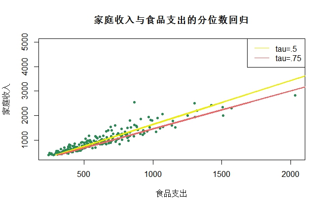

不同分位点的回归比较
fit = rq(foodexp ~ income,  tau = c(0.05,0.25,0.5,0.75,0.95), data = engel)
plot( summary(fit))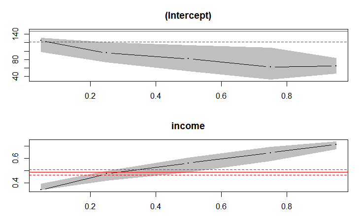

多元分位数回归

data(barro)

fit1 <- rq(y.net ~ lgdp2 + fse2 + gedy2 + Iy2 + gcony2, data = barro,tau=.25)
fit2 <- rq(y.net ~ lgdp2 + fse2 + gedy2 + Iy2 + gcony2, data = barro,tau=.50)
fit3 <- rq(y.net ~ lgdp2 + fse2 + gedy2 + Iy2 + gcony2, data = barro,tau=.75)
# 替代方式 fit <- rq(y.net ~ lgdp2 + fse2 + gedy2 + Iy2 + gcony2, method = "fn", tau = 1:4/5, data = barro)

anova(fit1,fit2,fit3)             # 不同分位点模型比较-方差分析
anova(fit1,fit2,fit3,joint=FALSE)
`
Quantile Regression Analysis of Deviance Table

Model: y.net ~ lgdp2 + fse2 + gedy2 + Iy2 + gcony2
Tests of Equality of Distinct Slopes: tau in {  0.25 0.5 0.75  }

       Df Resid Df F value  Pr(>F)  
lgdp2   2      481  1.0656 0.34535  
fse2    2      481  2.6398 0.07241 .
gedy2   2      481  0.7862 0.45614  
Iy2     2      481  0.0447 0.95632  
gcony2  2      481  0.0653 0.93675  
---
Signif. codes:  0 ‘***’ 0.001 ‘**’ 0.01 ‘*’ 0.05 ‘.’ 0.1 ‘ ’ 1
Warning message:
In summary.rq(x, se = se, covariance = TRUE) : 1 non-positive fis
`
不同分位点拟合曲线的比较
plot(barro$y.net,pch=20, col = "#2E8B57",
     main = "不同分位点拟合曲线的比较")
lines(fitted(fit1),lwd=2, col = "#FF00FF")
lines(fitted(fit2),lwd=2, col = "#EEEE00")
lines(fitted(fit3),lwd=2, col = "#EE6363")
legend("topright", c("tau=.25","tau=.50","tau=.75"), lty=c(1,1),
       col=c( "#FF00FF","#EEEE00","#EE6363"))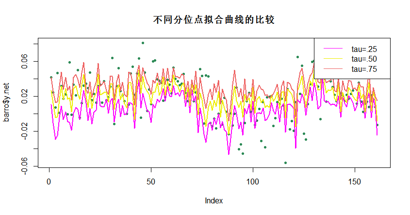

时间序列数据之动态线性分位数回归

library(zoo)
data("AirPassengers", package = "datasets")
ap <- log(AirPassengers)
fm <- dynrq(ap ~ trend(ap) + season(ap), tau = 1:4/5)
`
Dynamic quantile regression "matrix" data:
Start = 1949(1), End = 1960(12)
Call:
dynrq(formula = ap ~ trend(ap) + season(ap), tau = 1:4/5)

Coefficients:
                  tau= 0.2    tau= 0.4     tau= 0.6     tau= 0.8
(Intercept)    4.680165533  4.72442529  4.756389747  4.763636251
trend(ap)      0.122068032  0.11807467  0.120418846  0.122603451
season(ap)Feb -0.074408403 -0.02589716 -0.006661952 -0.013385535
season(ap)Mar  0.082349382  0.11526821  0.114939193  0.106390507
season(ap)Apr  0.062351869  0.07079315  0.063283042  0.066870808
season(ap)May  0.064763333  0.08453454  0.069344618  0.087566554
season(ap)Jun  0.195099116  0.19998275  0.194786890  0.192013960
season(ap)Jul  0.297796876  0.31034824  0.281698714  0.326054871
season(ap)Aug  0.287624540  0.30491687  0.290142727  0.275755490
season(ap)Sep  0.140938329  0.14399906  0.134373833  0.151793646
season(ap)Oct  0.002821207  0.01175582  0.013443965  0.002691383
season(ap)Nov -0.154101220 -0.12176290 -0.124004759 -0.136538575
season(ap)Dec -0.031548941 -0.01893221 -0.023048200 -0.019458814

Degrees of freedom: 144 total; 131 residual
`
sfm <- summary(fm)
plot(sfm)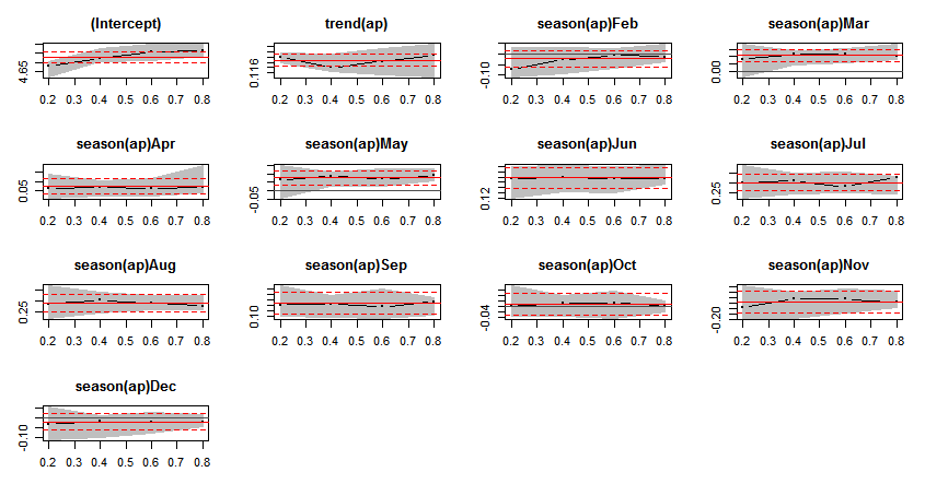

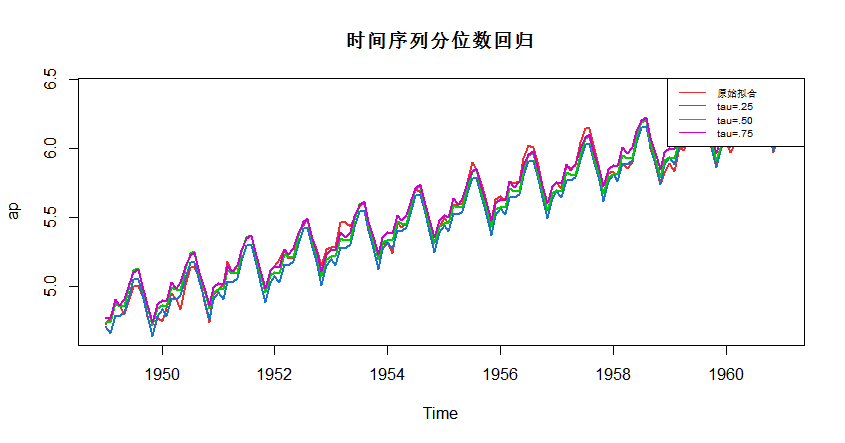
不同分位点拟合曲线的比较
fm1 <- dynrq(ap ~ trend(ap) + season(ap), tau = .25)
fm2 <- dynrq(ap ~ trend(ap) + season(ap), tau = .50)
fm3 <- dynrq(ap ~ trend(ap) + season(ap), tau = .75)

plot(ap,cex = .5,lwd=2, col = "#EE2C2C",main = "时间序列分位数回归")
lines(fitted(fm1),lwd=2, col = "#1874CD")
lines(fitted(fm2),lwd=2, col = "#00CD00")
lines(fitted(fm3),lwd=2, col = "#CD00CD")
legend("topright", c("原始拟合","tau=.25","tau=.50","tau=.75"), lty=c(1,1),
       col=c( "#EE2C2C","#1874CD","#00CD00","#CD00CD"),cex = 0.65)

除了本文介绍的以上内容，quantreg包还包含残差形态的检验、非线性分位数回归和半参数和非参数分位数回归等等，详细参见：用R语言进行分位数回归-詹鹏（北京师范大学经济管理学院）和Package ‘quantreg’。

反馈与建议

• 作者：ShangFR
• 邮箱：shangfr@foxmail.com