线性回归R实例

一、一元线性回归

以R中自带的trees数据集为例进【微软visual studio2017中R相关数据科学模块】

> head(trees)
Girth Height Volume#包含树龄、树高、体积
1 8.3 70 10.3
2 8.6 65 10.3
3 8.8 63 10.2
4 10.5 72 16.4
5 10.7 81 18.8
6 10.8 83 19.7

先绘制一下散点图，看看变量之间是否存在线性关系：体积、树龄

> library(ggplot2)
> qplot(x = log(Girth),y = log(Volume),data = trees,main = 'Volume and Girth Relation', colour = I('skyblue'),size = 10)

 有图得知，存在线性关系，进行建模

> model<-lm(Volume~Girth,data = trees)
> summary(model)

Call:
lm(formula = Volume ~ Girth, data = trees)

Residuals:#残差较大
   Min     1Q Median     3Q    Max 
-8.065 -3.107  0.152  3.495  9.587 

Coefficients:#系数的假设检验，P值都较小，在模型中呈显著状态***
            Estimate Std. Error t value Pr(>|t|)    
(Intercept) -36.9435     3.3651  -10.98 7.62e-12 ***
Girth         5.0659     0.2474   20.48  < 2e-16 ***
---
Signif. codes:  0 ‘***’ 0.001 ‘**’ 0.01 ‘*’ 0.05 ‘.’ 0.1 ‘ ’ 1

Residual standard error: 4.252 on 29 degrees of freedom
Multiple R-squared:  0.9353,    Adjusted R-squared:  0.9331 
F-statistic: 419.4 on 1 and 29 DF,  p-value: < 2.2e-16 #F统计量，也是显著的

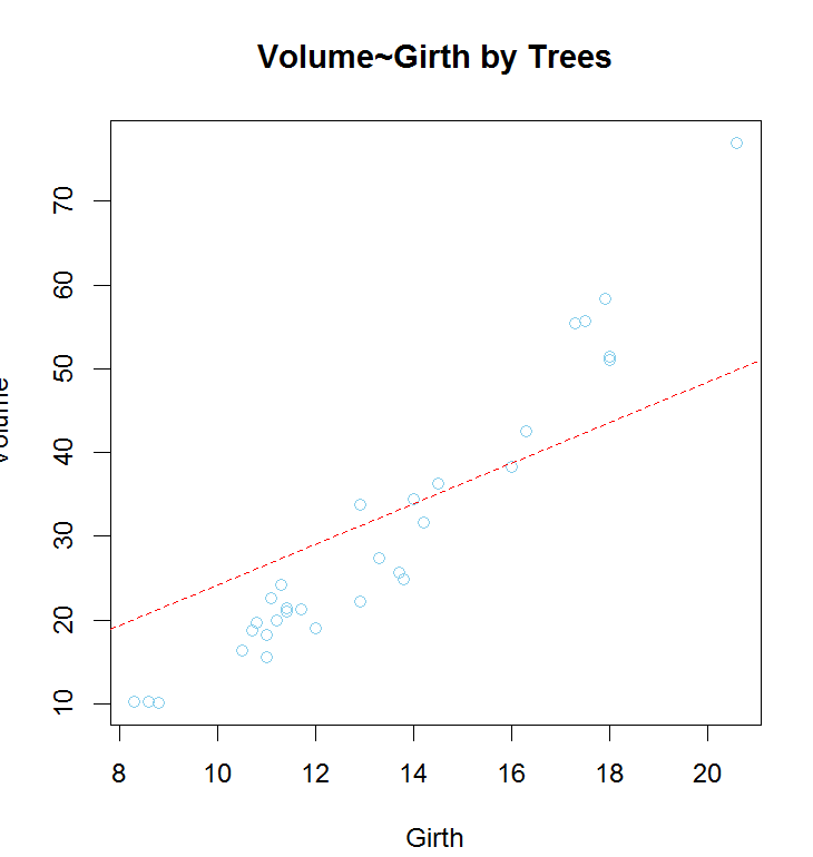
 将拟合直线绘制到原图上，查看拟合情况

> plot(Volume ~ Girth, data = trees,main = 'Volume and Girth Relation', col = 'skyblue')
+ abline(model, col = 'red', lty = 3)

但截距项不应该为负数（无论树龄再小体积也不应该为负数，就算只是一颗种子它也是有体积的），所以也可以用下面方法将截距强制为0：

> model <- lm(Volume ~ Girth - 1, data = trees)
+ summary(model)

Call:
lm(formula = Volume ~ Girth - 1, data = trees)

Residuals:#残差有所增大
    Min      1Q  Median      3Q     Max 
-11.104  -8.470  -6.199   1.883  27.129 

Coefficients:
      Estimate Std. Error t value Pr(>|t|)    
Girth   2.4209     0.1253   19.32   <2e-16 *** #截距项已经去除只剩树龄
---
Signif. codes:  0 ‘***’ 0.001 ‘**’ 0.01 ‘*’ 0.05 ‘.’ 0.1 ‘ ’ 1

Residual standard error: 9.493 on 30 degrees of freedom
Multiple R-squared:  0.9256,    Adjusted R-squared:  0.9231 
F-statistic: 373.1 on 1 and 30 DF,  p-value: < 2.2e-16

将现在的模型与之前的模型进行比较

也可以plot模型输出结果，评价模型效果

par(mfrow=c(2,2))
plot(model)

左上图是残差对拟合值作图，整体呈现出一种先下降后下升的模式，显示残差中可能还存在未提炼出来的影响因素。

右上图残差QQ图，用以观察残差是否符合正态分布。

左下图是标准化残差对拟合值，用于判断模型残差是否等方差。

右下图是标准化残差对杠杆值，虚线表示的cooks距离等高线。我们发现31号样本有较大的影响，需要进行变换。

plot(sqrt(Volume)~Girth,data=trees,pch=16,col='skyblue')#对整体进行开根号变换，线性趋势仍然明显

plot(log(Volume) ~ Girth, data = trees, pch = 16, col = 'red')#对整体进行log变换，

 与开根号趋势差异不大，采用开根号后变换重新进行建模

> model <- lm(sqrt(Volume) ~ Girth, data = trees)
+ summary(model)

Call:
lm(formula = sqrt(Volume) ~ Girth, data = trees)

Residuals:#整体残差明显变小
     Min       1Q   Median       3Q      Max 
-0.56640 -0.19429 -0.01169  0.20934  0.65575 

Coefficients:
            Estimate Std. Error t value Pr(>|t|)    
(Intercept) -0.55183    0.23719  -2.327   0.0272 *  
Girth        0.44262    0.01744  25.385   <2e-16 ***
---
Signif. codes:  0 ‘***’ 0.001 ‘**’ 0.01 ‘*’ 0.05 ‘.’ 0.1 ‘ ’ 1

Residual standard error: 0.2997 on 29 degrees of freedom
Multiple R-squared:  0.9569,    Adjusted R-squared:  0.9555 
F-statistic: 644.4 on 1 and 29 DF,  p-value: < 2.2e-16

> plot(sqrt(Volume) ~ Girth, data = trees, pch = 16, col = 'red')
+ abline(model, lty = 2)

其实跟最初拟合的效果差别不大

par(mfrow=c(2,2))
plot(model)

上图可知，原先的31号点已被削减，基本上没有太明显的异常点

预测使用时只需要输入建立模型名称以及数据框（包含X属性的列名，本列中即树龄），预测值为体积

> head(predict(model, trees))
       1        2        3        4        5        6 
3.121955 3.254743 3.343268 4.095729 4.184254 4.228516 

二、多元线性回归

与一元线性回归不同的是采用多个自变量来预测或者估计因变量

步骤与一元类似：

1、相关性检验，共线变量需要进行一定取舍，可以通过corrplot(cor(数据框名称))查看相关性

2、model <- lm(因变量~自变量1+自变量2+自变量3..., data = 数据框名称)进行建模，summary进行查看模型效果

3、同样可以用par(mfrow=c(2,2)）、plot(model)查看效果及异常点情况

4、根据结果进行调整，重新建模，直到获得较为满意的结果为止。

三、广义线性回归

基本语法

逻辑回归，再根据结果进行

model <- glm(因变量~自变量1 +自变量2 + 自变量3...,
             data = 数据框,
             family = binomial)

泊松回归：修改family

老师原文地址：https://notebooks.azure.com/YukWang/libraries/rDataAnalysis