机器学习培训

英伟达深度学习学院

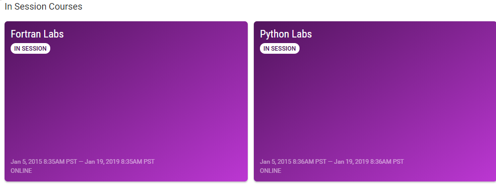
1现场培训：https://nvidia.qwiklab.com/my_learning

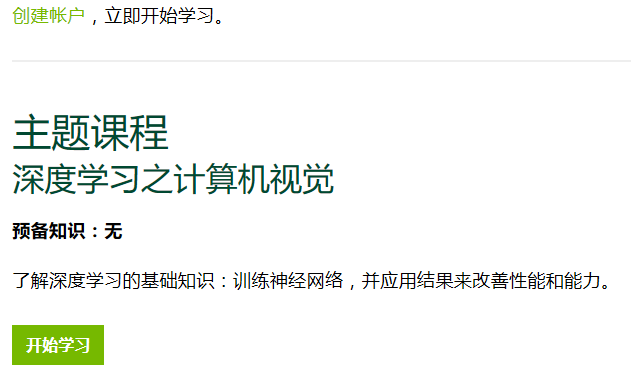
2课程连接：https://www.nvidia.com/zh-cn/deep-learning-ai/onlinelabs/?from=singlemessage 

3网易斯坦福

机器学习框架 

Python 带来的开发速度和 C++ 带来的执行速度。

caffe/caffe2

• Caffe846是一个清晰而高效的深度学习353框架，其作者是博士毕业于UC Berkeley的贾扬清2.2K，目前在Google148工作。
• Caffe76是纯粹的C++/CUDA架构，支持命令行、Python和MATLAB接口；可以在CPU和GPU201直接无缝切换： 

TensorFlow 谷歌开源框架

MXnet

(2016年6月27日更新)大半年的时间过去了，再回过头来看这篇文章，感觉有点伤感，Caffe已经很久没有更新过了，曾经的霸主地位果然还是被tensorflow给终结了，特别是从0.8版本开始，tensorflow开始支持分布式，一声叹息…MXNet还是那么拼命，支持的语言新增了四种，Matlab/Javascripts/C++/Scala，文档也变的更漂亮了，还推出了手机上图片识别的demo[8]。

固件和部署应用

https://nvidia.qwiklab.com/focuses/5866

 

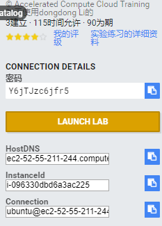
 直接回到数据集和模型建立界面

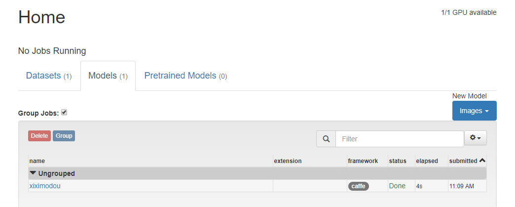
1建立数据集

2设置参数 彩色或黑白

3 选择数据地址

小心空格

 4 为数据集起名字

 建立第二个数据集

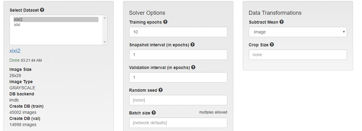
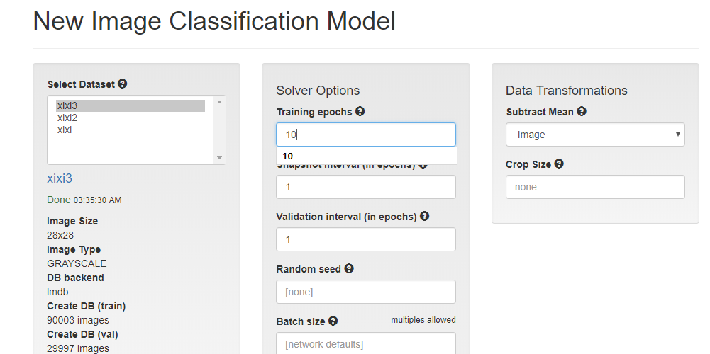
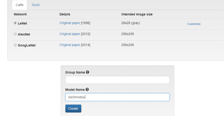
 建立模型

层数选择10

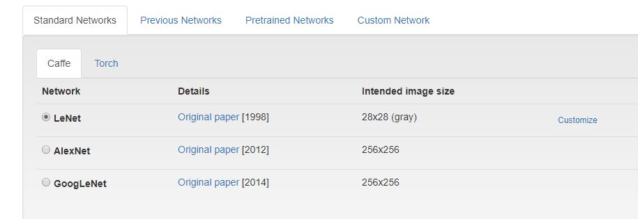
网络模型选择

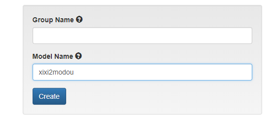
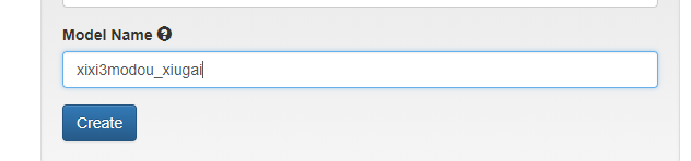
名字

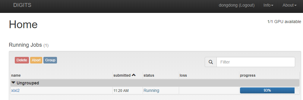
开始运行

测试图片

输入测试图片，点击 classify 执行

 结果

测试多张图片 

回到教程，选择下一步

找到代码 ，选中  按 shift +enter

 保存

/notebooks/test_images/image-1-1.jpg
/notebooks/test_images/image-2-1.jpg
/notebooks/test_images/image-3-1.jpg
/notebooks/test_images/image-4-1.jpg
/notebooks/test_images/image-7-1.jpg
/notebooks/test_images/image-8-1.jpg
/notebooks/test_images/image-8-2.jpg

保存tet文件

上传 开始

提高模型，增大数据集

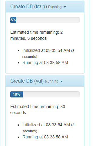
 等待运行完

 

加载有点慢

 新建模型

 

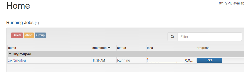
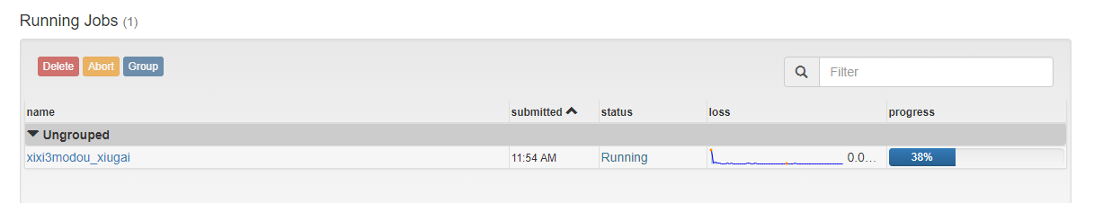
 开训练

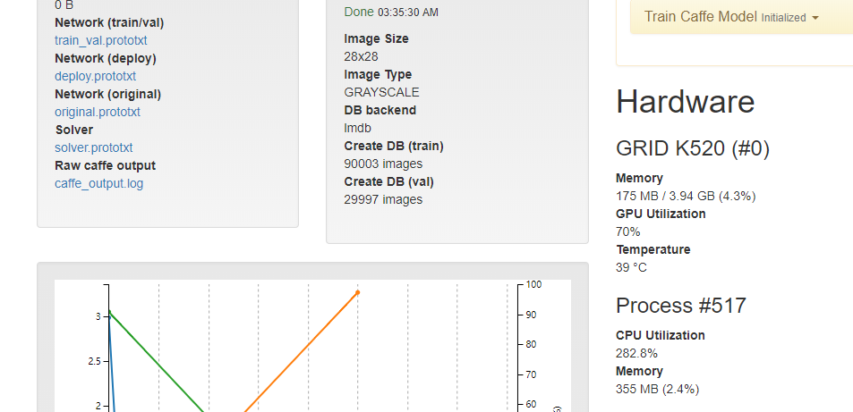
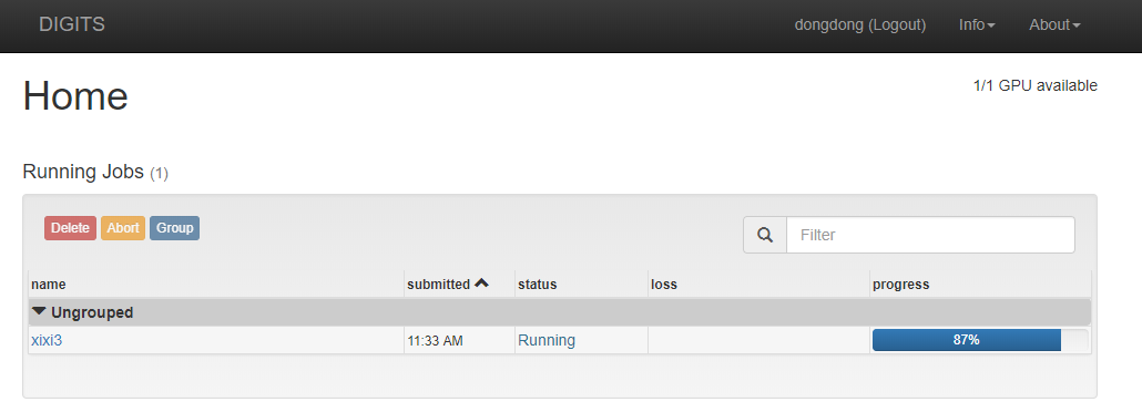
主界面告诉你训练时间

训练完，使用测试图实验

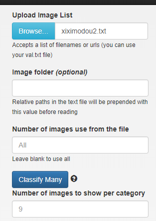
上传图片路径 txt文件  测试多张图片

 

选择新的开始按钮

结果

 

也可以自己手写，画板 大小保存成 28*28

打开画板

点击下方

 网络模型优化

选中模型克隆

 

 可观看可视化的图

 （上图绿色模块为下面添加的层）

 67 {}  最后面 加入一层

layer {
  name: "reluP1"
  type: "ReLU"
  bottom: "pool1"
  top: "pool1"
}      

 改为 75

 改为 100

 保存修改后的模型

重新开始识别上传手写字符

 

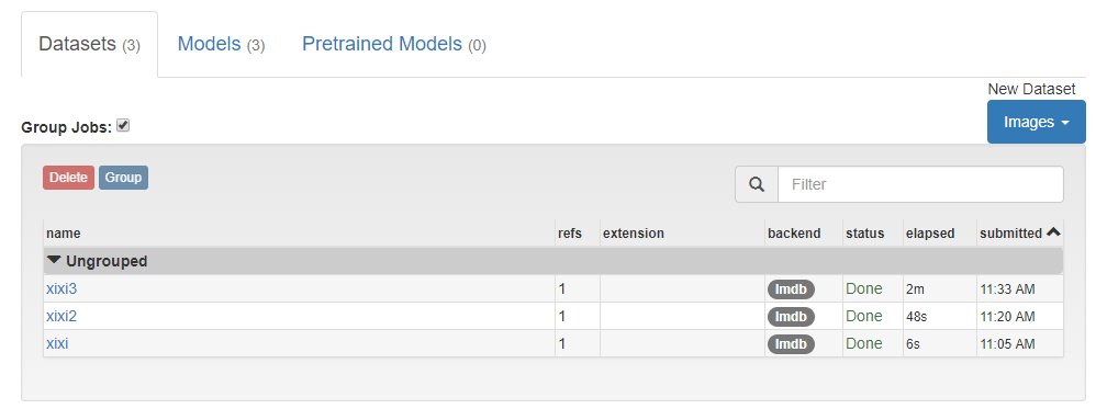
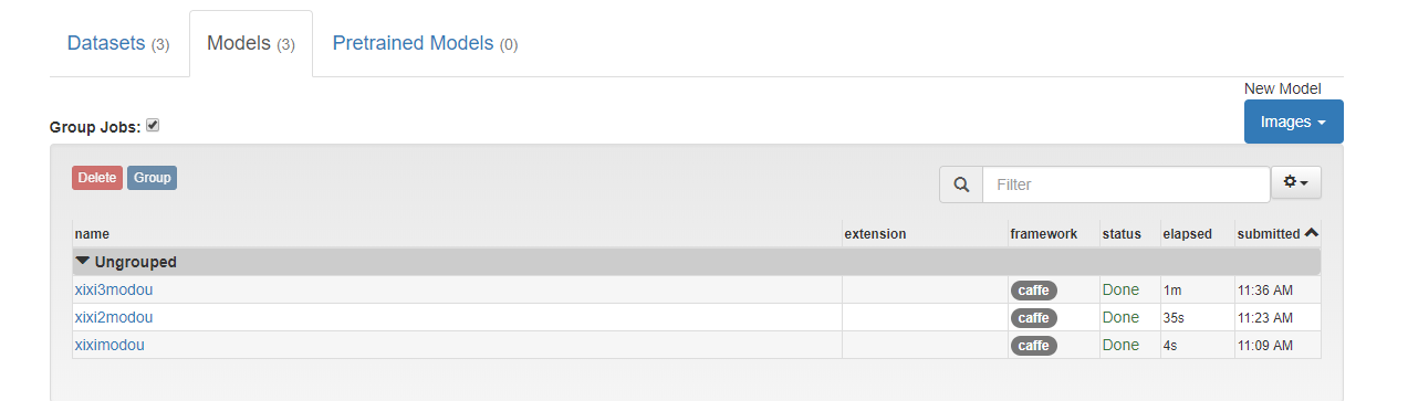
 目前为止我们所有创建的数据集和模型

教程 https://medium.com/@dmonn/how-to-use-nvidia-digits-for-image-classification-79600acbe0db

https://www.leiphone.com/news/201706/k7eKW8nLuKtZA2NG.html

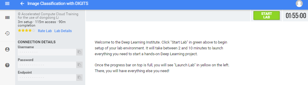
Image Classification with DIGITS

                                 An introduction to Deep Learning

 

In this lab, you'll learn to train a neural network using clean labeled data. We'll introduce deep learning through the task of supervised image classification, where, given many images and their labels, you'll build a tool that can predict labels of newimages.

The intent is to build the skills to start experimenting with deep learning. You'll examine:

• What it means to train vs. to program
• The role of data in artificial intelligence
• How to load data for training a neural network
• The role of a network in deep learning
• How to train a model with data

At the end of this lab, you'll have a trained neural network that can successfully classify images to solve a classic deep learning challenge:

How can we digitize handwriting?

 

Training vs. programming

The fundamental difference between artificial intelligence (AI) and traditional programing is that AI learns while traditional algorithms are programmed. Let's examine the difference through an example:

Imagine you were asked to give a robot instructions to make a sandwich using traditional computer programming, instruction by instruction. How might you start?

Maybe something like:
Add two pieces of bread to an empty plate.

Run the code below to see what the robot might do with your first instruction. To run code, click on In [ ] and press Shift + Enter.

In [ ]:

 

 

 

 

 

readyPlate = 2*bread + emptyPlate

 

 

 

You likely got a "NameError." How would you then work to define "bread" to your robot? Not to mention other ingredients and how to combine them?

Computers only "see" images as the amount of red, blue, and green at each pixel. Everything else we want them to know, we would have had to describe in terms of pixels.

 

Artificial intelligence takes a different approach. Instead of providing instructions, we provide examples. Above, we could showour robot thousands of labeled images of bread and thousands of labeled images of other objects and ask our robot to learn the difference. Our robot could then build its own program to identify new groups of pixels (images) as bread.

Instead of instructions, we now need data and computers designed to learn.

The Big Bang in Machine Learning

• Data: In the era of big data, we create ~2.5 quintillion bytes of data per day. Free datasets are available from places like Kaggle.com and UCI. Crowdsourced datasets are built through creative approaches - e.g. Facebook asking users to "tag" friends in their photos to create labeled facial recognition datasets. More complex datasets are generated manually by experts - e.g. asking radiologists to label specific parts of the heart.
• Computers designed to learn - software: Artificial neural networks are inspired by the human brain. Like their biological counterparts, they are structured to understand (and represent) complex concepts, but their biggest strength is their ability to learn from data and feedback. The "deep" in deep learning refers to many layers of artificial neurons, each of which contribute to the network's performance.
• Computers designed to learn - hardware: The computing that powers deep learning is intensive, but not complex. Processing huge datasets through deep networks is made possible by parallel processing, a task tailor made for the GPU.

So how do we expose artificial neural networks to data?

By the end of this lab, you'll know how to load data into a deep neural network to create a trained model that is capable of solving problems with what it learned, not what a programmer told it to do.

 

Training a network to recognize handwritten digits

Since a computer "sees" images as collections of pixel values, it can't do anything with visual data unless it learns what those pixels represent.

What if we could easily convert handwritten digits to the digital numbers they represent?

1. We could help the post office sort piles of mail by post code. This is the problem that motivated Yann LeCun. He and his team put together the dataset and neural network that we'll use today and painstakingly pioneered much of what we know now about deep learning.
2. We could help teachers by automatically grading math homework. This the problem that motivated the team at answer.ky, who used Yann's work to easily solve a real world problem using a workflow like what we'll work through now.
3. We could solve countless other challenges. What will you build?

We're going to train a deep neural network to recognize handwritten digits 0-9. This challenge is called "image classification," where our network will be able to decide which image belongs to which class, or group.

For example:
The following image should belong to the class '4':

 

whereas this next image should belong to the class '2':

 

It's important to note that this workflow is common to most image classification tasks, and is a great entry point to learning how to solve problems with Deep Learning.

Let's start.

Load and organize data

Let's start by bringing our data, in this case, thousands of images, into our learning environment. We're going to use a tool called DIGITS, where we can visualize and manage our data.

First, open DIGITS in a new tab using the following link.

Open DIGITS.

Loading our first dataset

When you start DIGITS, you will be taken to the home screen where you can create new datasets or new models.

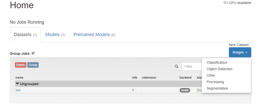
Begin by selecting the Datasets tab on the left.

Since we want our network to tell us which "class" each image belongs to, we ask DIGITS to prepare a "classification" image dataset by selecting "Classification" from the "Images" menu on the right.

At this point you may need to enter a username. If requested, just enter any name in lower-case.

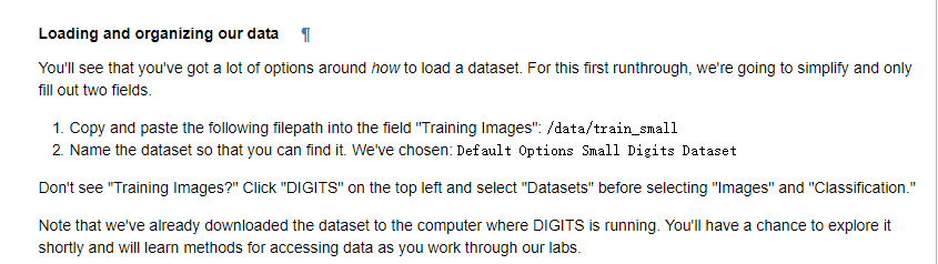
Loading and organizing our data

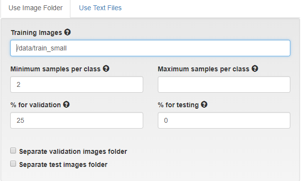
You'll see that you've got a lot of options around how to load a dataset. For this first runthrough, we're going to simplify and only fill out two fields.

1. Copy and paste the following filepath into the field "Training Images": /data/train_small
2. Name the dataset so that you can find it. We've chosen: Default Options Small Digits Dataset

Don't see "Training Images?" Click "DIGITS" on the top left and select "Datasets" before selecting "Images" and "Classification."

Note that we've already downloaded the dataset to the computer where DIGITS is running. You'll have a chance to explore it shortly and will learn methods for accessing data as you work through our labs.

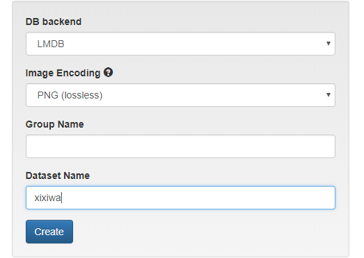
Then press "Create."

DIGITS is now creating your dataset from the folder. Inside the folder train_small there were 10 subfolders, one for each class (0, 1, 2, 3, ..., 9). All of the handwritten training images of '0's are in the '0' folder, '1's are in the '1' folder, etc.

Explore what our data looks like by selecting "Explore the db".

Your data

While there is an endless amount of analysis that we could do on the data, make sure you at least note the following:

1. This data is labeled. Each image in the dataset is paired with a label that informs the computer what number the image represents, 0-9. We're basically providing a question with its answer, or, as our network will see it, a desired output with each input. These are the "examples" that our network will learn from.
2. Each image is simply a digit on a plain background. Image classification is the task of identifying the predominant object in an image. For a first attempt, we're using images that only contain one object. We'll build skills to deal with messier data in subsequent labs.

This data comes from the MNIST dataset which was created by Yann LeCun. It's largely considered the "Hello World," or introduction, to deep learning.

Learning from our data - Training a neural network

Next, we're going to use our data to train an artificial neural network. Like its biological inspiration, the human brain, artificial neural networks are learning machines. Also like the brain, these "networks" only become capable of solving problems with experience, in this case, interacting with data. Throughout this lab, we'll refer to "networks" as untrained artificial neural networks and "models" as what networks become once they are trained (through exposure to data).

For image classification (and some other tasks), DIGITS comes pre-loaded with award-winning networks. As we take on different challenges in subsequent labs, we'll learn more about selecting networks and even building our own. However, to start, weighing the merits of different networks would be like arguing about the performance of different cars before driving for the first time. Building a network from scratch would be like building your own car. Let's drive first. We'll get there.

Go to the tab where DIGITS is still open and return to the main screen by clicking "DIGITS" on the top left of the screen.

Creating a new model in DIGITS is a lot like creating a new dataset. From the home screen, the "Models" tab will be pre-selected. Click "Images" under "New Model" and select "Classification", as we're creating an image classification model to match our image classification dataset and image classification task.

Again, for this first round of training let's keep it simple. The following are the fewest settings you could possibly set to successfully train a network.

1. We need to choose the dataset we just created. Select our Default Options Small Digits Dataset dataset.
2. We need to tell the network how long we want it to train. An epoch is one trip through the entire training dataset. Set the number of Training Epochs to 5 to give our network enough time to learn something, but not take all day. This is a great setting to experiment with.
3. We need to define which network will learn from our data. Since we stuck with default settings in creating our dataset, our database is full of 256x256 color images. Select the network AlexNet, if only because it expects 256x256 color images.
4. We need to name the model, as hopefully we'll do a lot of these. We chose My first model.

When you have set all of these options, press the Create button.

You are now training your model! For this configuration, the model training should complete in less than 5 minutes. You can either watch it train, continue reading, or grab a cup of coffee.

When done, the Job Status on the right will say "Done", and your training graph should look something like:

We'll dig into this graph as a tool for improvement, but the bottom line is that after 5 minutes of training, we have built a model that can map images of handwritten digits to the number they represent with an accuracy of about 87%!

Let's test the ability of the model to identify new images.

Inference

Now that our neural network has learned something, inference is the process of making decisions based on what was learned. The power of our trained model is that it can now classify unlabeled images.

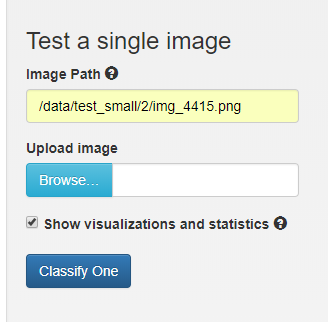
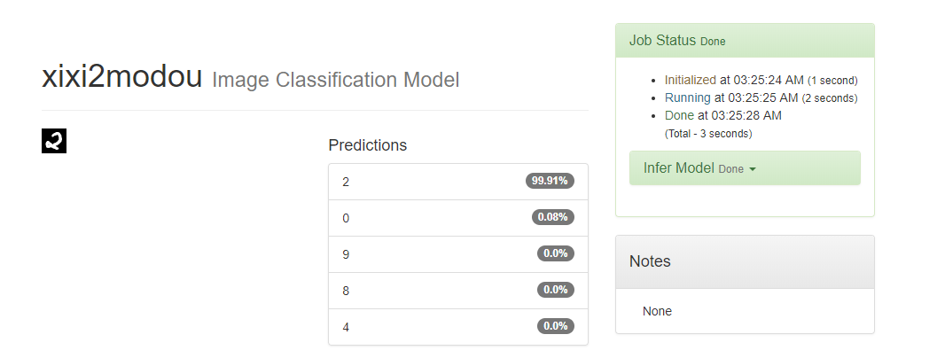
We'll use DIGITS to test our trained model. At the bottom of the model window, you can test a single image or a list of images. On the left, type in the path /data/test_small/2/img_4415.png in the Image Path text box. Select the Classify One button. After a few seconds, a new window is displayed with the image and information about its attempt to classify the image.

 

It worked! (Try again if it didn't). You took an untrained neural network, exposed it to thousands of labeled images, and it now has the ability to accurately predict the class of unlabeled images. Congratulations!

Note that that same workflow would work with almost any image classification task. You could train AlexNet to classify images of dogs from images of cats, images of you from images of me, etc. If you have extra time at the end of this lab, theres another dataset with 101 different classes of images where you can experiment.

While you have been successful with this introductory task, there is a lot more to learn.

In the next notebook, you will work to define and improve performance.

 

Continue to the next notebook

 

第二个教程

Improving your Model

 

Now that you've learned to successfully train a model, let's work to train a state of the art model. In this lab, we'll learn the levers that you, as a deep learning practitioner, will use to navigate towards desired results. In the process, we'll start to peel back the layers around the technology that makes this possible.

Let's bring back our handwritten digit classifier. Go to DIGITS' home screen by clicking the DIGITS logo on the top left of the screen. Here, you'll see (at least) two models. Choose the first model you created, in our case, "My first model."

Among other things, DIGITS will display the graph that was generated as the model was being trained.

Three quantities are reported: training loss, validation loss, and accuracy. The values of training and validation loss should have decreased from epoch to epoch, although they may jump around some. The accuracy is the measure of the ability of the model to correctly classify the validation data. If you hover your mouse over any of the data points, you will see its exact value. In this case, the accuracy at the last epoch is about 87%. Your results might be slightly different than what is shown here, since the initial networks are generated randomly.

Analyzing this graph, one thing that jumps out is that accuracy is increasing over time and that loss is decreasing. A natural question may be, "will the model keep improving if we let it train longer?" This is the first intervention that we'll experiment with and discuss.

Study more

Following the advice of parents and teachers everywhere, let's work to improve the accuracy of our model by asking it to study more.

An epoch is one complete presentation of the data to be learned to a learning machine. Let's make sense of what is happening during an epoch.

1. Neural networks take the first image (or small group of images) and make a prediction about what it is (or they are).
2. Their prediction is compared to the actual label of the image(s).
3. The network uses information about the difference between their prediction and the actual label to adjust itself.
4. The network then takes the next image (or group of images) and make another prediction.
5. This new (hopefully closer) prediction is compared to the actual label of the image(s).
6. The network uses information about the difference between this new prediction and the actual label to adjust again.
7. This happens repeatedly until the network has looked at each image.

Compare this to a human study session using flash cards:

1. A student looks at a first flashcard and makes a guess about what is on the other side.
2. They check the other side to see how close they were.
3. They adjust their understanding based on this new information.
4. The student then looks at the next card and makes another prediction.
5. This new (hopefully closer) prediction is compared to the answer on the back of the card.
6. The student uses information about the difference between this new prediction and the right answer to adjust again.
7. This happens repeatedly until the student has tried each flashcard once.

You can see that one epoch can be compared to one trip through a deck of flashcards.

In the model that we trained, we asked our network for 5 epochs. The blue curve on the graph above shows how far off each prediction was from the actual label.

Like a human student, the point of studying isn't just to be able to replicate someone else's knowledge. The green curve shows the difference between the model's predictions and actual labels for NEW data that it hasn't learned from. The orange curve is simple the inverse of that loss.

Loss can be measured in many ways, but conceptually, it's simply the difference between predicted and actual labels.

If after taking a test and earning 87%, a human student wanted to improve performance, they might be advised to study more. At this point, they'd go back to their flashcards.

A deep learning practitioner could request more epochs. It is possible to start from scratch and request more epochs when creating your model for the first time. However, our model has already spent some time learning! Let's use what it has learned to improve our model instead of start from scratch.

Head back to DIGITS and scroll to the bottom of your model page and click the big green button labeled: "Make Pretrained Model."

This will save two things:

1. The "network architecture" that you chose when selecting "AlexNet."
2. What the model has "learned" in the form of the parameters that have been adjusted as your network worked through the data in the first 5 epochs.

We can now create a new model from this starting point. Go back to DIGITS' home screen and create a new Image Classfication model like before. New Model (Images) -> Classification

• Select the same dataset - (Default Options Small Dataset)
• Choose some number of epochs between 3 and 8. (Note that in creating a model from scratch, this is where you could have requested more epochs originally.)
• This time, instead of choosing a "Standard Network," select "Pretrained Networks."
• Select the pretrained model that you just created, likely "My first model."
• Name your model - We chose "Study more"
• Click Create

Your settings should look like:

When you create the model, you'll get the following graph.

Note the following:

1. As expected, the accuracy starts close to where our first model left off, 86%.
2. Accuracy DOES continue to increase, showing that increasing the number of epochs often does increase performance.
3. The rate of increase in accuracy slows down, showing that more trips through the same data can't be the only way to increase performance.

Let's test our new and improved model using the same image from before. At the bottom of our model page, "Test a single image." We'll test the same "2" to compare performance. As a reminder, the image path is:
/data/test_small/2/img_4415.png

Recall that our original model correctly identified this as a 2 as well, but with a confidence of 85%. This is clearly a better model.

Feel free to try a few more images by changing the number after "img_ "

 

Let's try testing the model with a set of images. They are shown below.

image-1-1.jpg

image-2-1.jpg

image-3-1.jpg

image-4-1.jpg

image-7-1.jpg

image-8-1.jpg

image-8-2.jpg

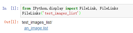
We can classify multiple files if we put them in the list. In the link below, execute the code block and a link to the file an_image.list will appear. Right click on an_image.list and save that to a file on your local computer(right click and "Save As"). Remember the directory in which it is saved.

In [ ]:

 

 

 

 

 

from IPython.display import FileLink, FileLinks

FileLinks('test_images_list')

 

 

 

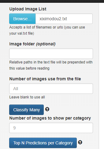
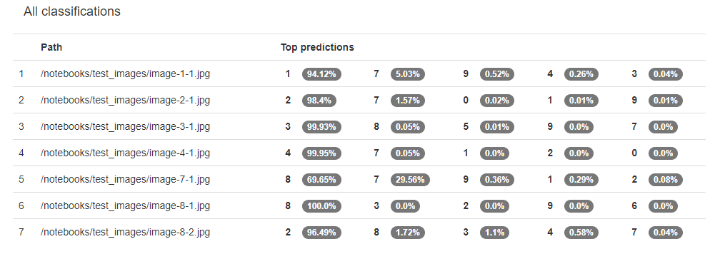
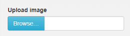
On the right side of the DIGITS model page, there is an option to "test a list of images". Press the button Browse and select the an_image.list file you just downloaded. Then press the Classify Many button. After several seconds, you will see the results from Caffe trying to classify these images with the generated model. In the image name, the first number is the digit in the image (ex. image-3-1.jpg is a 3). Your results should be similar to this:

What is shown here is the probability that the model predicts the class of the image. The results are sorted from highest probability to lowest. Our model didn't do so well.

While the accuracy of the model was 87%, it could not correctly classify any of the images that we tested. What can we do to improve the classification of these images?

 

At this point it's time to be a bit more intentional. After we can successfully train a model, what comes next comes from understanding and experimentation. To build a better understanding of THIS project, we should start with our data. To build a better understanding of anything, we should start with primary sources.

The dataset that we are learning from is a subset of the MNIST dataset. A close read of the documentation would likely yield a lot of insight.

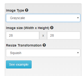
One key observation we'll use is that the images start as 28x28 grayscale images. When we loaded our dataset, we stuck with defaults, which were 256x256 and color. You may have noticed that the images were a bit blurry. In the next section we'll explore the benefits that can come from matching your data to the right model.

The right model

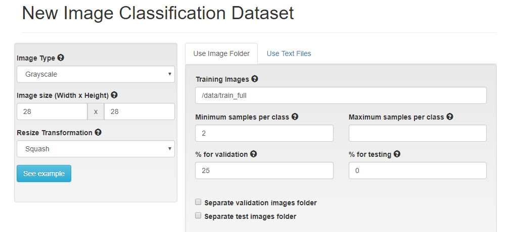
Let's start from scratch using what we've learned. This time, we'll load our data as 28x28 grayscale images and pick a model that is built to accept that type of data, LeNet. To compare to our previous model, use the total number of epochs that you trained with so far, eg. the 5 in "my first model" and the additional epochs trained from your pretrained model. In my case I'll use 8.

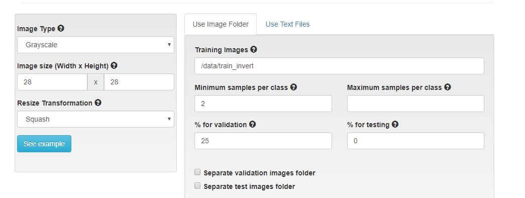
Here's an image of the settings that would create the dataset.

Feel free to "explore the db" again. I notice immediately that the images are no longer blurry.

Next, create a model using the settings in the image below. Note that the LeNet model is designed to take 28x28 grayscale images. You'll see shortly that this network was actually purpose-built for digit classification.

Woah. You should have noticed two things.

1. Your model improved performance. Mine was accurate to more than 96%.
2. Your model trained faster. In far less than two minutes, my model ran through 8 epochs.

We haven't done anything to address the problem of more diverse data, but if we can train faster, we can experiment a lot more.

 

Train with more data

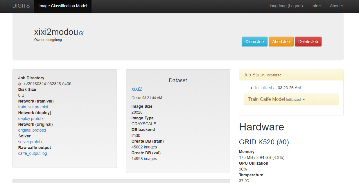
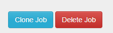
In our last attempt at training, we only used 10% of the full MNIST dataset. Let's try training with the complete dataset and see how it improves our training. We can use the clone option in DIGITS to simplify the creation of a new job with similar properties to an older job. Let's return to the home page by clicking on DIGITS in the upper left corner. Then select Dataset from the left side of the page to see all of the datasets that you have created. You will see your Mnist small dataset. When you select that dataset, you will be returned to the results window of that job. In the right corner you will see a button: Clone Job.

Press the Clone Job button.

From here you will see the create dataset template populated with all the options you used when you created the Default Options Small Digits dataset. To create a database with the full MNIST data, change the following settings:

• Training Images - /data/train_full
• Dataset Name - MNIST full

Then press the Create button. This dataset is ten times larger than the other dataset, so it will take a few minutes to process.

After you have created your new database, follow the same procedure to clone your training model. In the template, change the following values:

• Select the MNIST full dataset
• Change the name to MNIST full

Then create the model.

With much more data, the model will take longer to run. It still should complete in less than a minute. What do you notice that is different about the results? Both the training and validation loss function values are much smaller. In addition, the accuracy of the model is around 99%, possibly greater. That is saying the model is correctly identifying most every image in its validation set. This is a significant improvement. However, how well does this new model do on the challenging test images we used previously?

Using the same procedure from above to classify our set of test images, here are the new results:

The model was still only able to classify one of the seven images. While some of the classifications came in a close second, our model's predictive capabilities were not much greater. Are we asking too much of this model to try and classify non-handwritten, often colored, digits with our model?

 

Improving Model Results - Data Augmentation

You can see with our seven test images that the backgrounds are not uniform. In addition, most of the backgrounds are light in color whereas our training data all have black backgrounds. We saw that increasing the amount of data did help for classifying the handwritten characters, so what if we include more data that tries to address the contrast differences?

Let's try augmenting our data by inverting the original images. Let's turn the white pixels to black and vice-versa. Then we will train our network using the original and inverted images and see if classification is improved.

To do this, follow the steps above to clone and create a new dataset and model. The directories for the augmented data are:

• Training Images - /data/train_invert

Remember to change the name of your dataset and model. When the new dataset is ready, explore the database. Now you should see images with black backgrounds and white numbers and also white backgrounds and black numbers.

Now train a new model. Clone your previous model results, and change the dataset to the one you just created with the inverted images. Change the name of the model and create a new model. When the training is complete, the accuracy hasn't really increased over the non-augmented image set. In fact, the accuracy may have gone down slightly. We were already at 99% so it is unlikely we were going to improve our accuracy. Did using an augmented dataset help us to better classify our images? Here is the result:

By augmenting our dataset with the inverted images, we could identify six of the seven images. While our result is not perfect, our slight change to the images to increase our dataset size made a significant difference.

 

Advanced - Improving Model Results by Modifying the Network (Optional)

Augmenting the dataset improved our results, but we are not identifying all our test images. Let's try modifying the LeNet network directly. You can create custom networks to modify the existing ones, use different networks from external sources, or create your own. To modify a network, select the Customize link on the right side of the Network dialog box.

This will open an editor with the LeNet model configuration. Scroll through the window and look at the code. The network is defined as a series of layers. Each layer has a name that is a descriptor of its function. Each layer has a top and a bottom, or possibly multiples of each, indicating how the layers are connected. The type variable defined what type the layer is. Possibilities include Convolution, Pool, and ReLU. All the options available in the Caffe model language are found in the Caffe Tutorial.

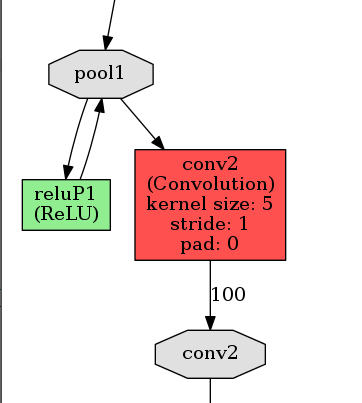
At the top of the editor, there is a Visualize button. Pressing this button will visualize all of the layers of the model and how they are connected. In this window, you can see that the data are initially scaled, there are two sets of Convolution and Pooling layers, and two Inner Products with a Rectilinear Unit (ReLU) connected to the first Inner Product. At the bottom of the network, there are output functions that return the accuracy and loss computed through the network.

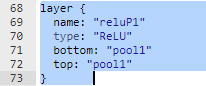
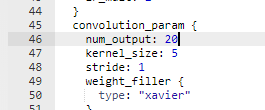
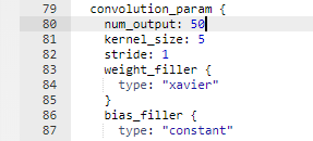
We are going to make two changes to the network. First, we are going to connect a ReLU to the first pool. Second, we are going to change the values of num_output to 75 for the first Convolution (conv1) and 100 for the second Convolution (conv2). The ReLU layer definition should go below the pool1 definition and look like:


layer {
  name: "reluP1"
  type: "ReLU"
  bottom: "pool1"
  top: "pool1"
}


The Convolution layers should be changed to look like:


layer {
  name: "conv1"
  type: "Convolution"
  bottom: "scaled"
  top: "conv1"
...
  convolution_param {
    num_output: 75
...

layer {
  name: "conv2"
  type: "Convolution"
  bottom: "pool1"
  top: "conv2"
...
  convolution_param {
    num_output: 100
...
Note, the ellipis (...) just indicates we removed some of the lines from the layer for brevity. The only change you have to make is to the value of num_output.

After making these changes, visualize your new model. You should see the ReLU unit appear similar to:

Now change the name of the model and press the Create button. When it is complete test the data again. The results should be similar to:

Were you able to correctly identify them all? If not, why do you think the results were different?

 

Next Steps

In our example here, we were able to identify most of our test images successfully. However, that is generally not the case. How would go about improving our model further? Typically, hyper-parameter searches are done to try different values of model parameters such as learning-rate or different solvers to find settings that improve model accuracy. We could change the model to add layers or change some of the parameters within the model associated with the performance of the convolution and pooling layers. In addition, we could try other networks.

 

Summary

In this tutorial you were introduced to Deep Learning and all of the steps necessary to classify images including data processing, training, testing, and improving your network through data augmentation and network modifications. In the training phase, you learned about the parameters that can determine the performance of training a network. By training a subset of the MNIST data, a full set, different models, augemented data, etc. you saw the types of options you have to control performance. In testing our model, we found that although the test images were quite different than the training data, we could still correctly classify them.

Now that you have a basic understanding of Deep Learning and how to train using DIGITS, what you do next is limited only by your own imagination. Test what you have learned, there are several good datasets with which to practice. We have included the CalTech 101 dataset at

/data/101_ObjectCategories

Feel free to run any part of this lab again with that (more complex) dataset.

There is still much more to learn! Start a Deep Learning project or take another course. The Nvidia Deep Learning Institute has a comprehensive library of hands-on labs for both fundamental and advanced topics.

 

 

Appendix

For a high performing and generalizable model:

1. Load the dataset stored at

   /data/train_invert

   as 28x28 grayscale images.

2. Train a model using the LeNet network for 5 epochs.