Live variable analysis
In compiler theory, live variable analysis(or simply livenesss analysis) is a classic data-flow analysis performed by compilers to calculate for each program point the variables that may be potentially read before their next write, that is, the variables that are live at the exit from each program point.
stated simply: a variable is live if it holds a value that may be needed in the future.
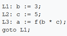
Example:
The set of live variables at line L3 is {b,c} because both are used in the multiplication, and thereby the call to f and assignment to a. But the set of live variables at line L1 is only {b} since variable c is updated in L2. The value of variable a is never used. Note that f may be stateful, so the never-live assignment to a can be eliminated, but there is insufficient information to rule on the entirely of L3.
Expression in terms of dataflow equations
Liveness analysis is a "backwards may" analysis. The analysis is done in a backwards order, and the dataflow confluence operator is set union. In other words, if applying liveness analysis to a function with a particular number of logical branches within it, the analysis is performed starting from the end of the function working towards the beginning(hence "backwards"), and a variable is considered live if any of the branches moving forward within the function might potentially(hence "may") need the variable's current value. This is in contrast to a "backwards must" analysis which would instead enforces this condition on all branches moving forwards.
The dataflow equations used for a given basic block s and exiting block f in live variable analysis are the following:
GEN[s]: The set of variables that are used in s before any assignment..
KILL[s]: The set of variables that are assigned a value in s(in many books, KILL(s) is also defined as the set of variables assigned a value in s before any use, but this does not change the solution of the dataflow equation):

The in-state of a block is the set of variables that are live at the start of the bock. Its out-state is the set of variables that are live at the end of if. The out-state is the union of the in-states of the block's sucessors. The transfer function of a statement is applied by making the variables that are writtern dead, then making the variables that are read live.
Second example
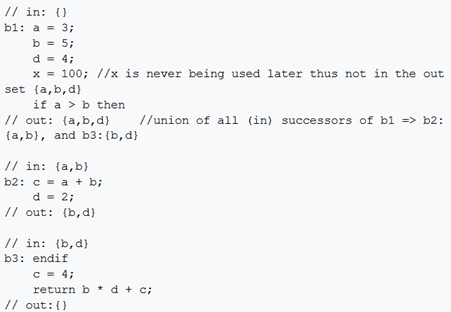
The in-state of b3 only contains b and d, since c has been writtern. The out-state of b1 is the union of the in-state of b2 and b3. The definition of c in b2 can be removed, since c is not live immediately after the statement.
Solving the data flow equations starts with initializing all in-state and out-states to the empty set. The work list is initialized by inserting the exit point(b3) in the work list(typical for backward flow). Its computed in-state differs from the previous one, so its predecessors b1 and b2 are inserted and the process continues. The progress is summarized in the table below.

Note that b1 was entered in the list before b2, which forced processing b1 twich(b1 was re-entered as processor of b2). Inserting b2 before b1 would have allowed earlier completion.