RNN and Language modeling in TensorFlow

RNNs and Language modeling in TensorFlow

From feed-forward to Recurrent Neural Networks (RNNs)

In the last few weeks, we've seen how feed-forward and convolutional neural networks have achieved incredible results. They perform on par with, even outperform, humans in many different tasks.

Despite their seemingly magical properties, these models are still very limited. Humans aren't built to just do linear or logistic regression, or recognize individual objects. We can understand, communicate, and create. The inputs we deal with aren't just singular data points, but sequences that are rich in information and complex in time dependencies. Languages we use are sequential. Music we listen to is sequential. TV shows we watch are sequential. The question is: how can we make our models capable of processing sequences of inputs with all their intricacies the way humans do.

RNNs were created with the aim of capturing the sequential information. The Simple Recurrent Network (SRN) was first introduced by Jeff Elman in a paper entitled "Finding structure in time" (Elman, 1990). As Professor James McClelland wrote in his book:

"The paper was groundbreaking for many cognitive scientists and psycholinguists, since it was the first to completely break away from a prior commitment to specific linguistic units (e.g. phonemes or words), and to explore the vision that these units might be emergent consequences of a learning process operating over the latent structure in the speech stream. Elman had actually implemented an earlier model in which the input and output of the network was a very low-level spectrogram-like representation, trained using a spectral information extracted from a recording of his own voice saying 'This is the voice of the neural network'."

RNNs are built on the same computational unit, known as neuron, as the feed-forward neural networks. However, they differ in the way these neurons are connected to one another. Feed forward neural networks are organized in layers: signals are passed in one direction only (from inputs to outputs) and loops aren't allowed. RNNs, on the contrary, allow neurons to connect to themselves. This allows for the notion of time to be taken into account, as the neuron from the previous step can affect the neuron at the current step.

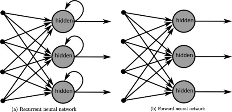
Graph from "A survey on the application of recurrent neural networks to statistical language modeling." by De Mulder et al. Computer Speech & Language 30.1 (2015): 61-98.

Elman's SRN did exactly this. In his early model, the hidden layer at this current step is a function of both the input at that step, and the hidden layer from the previous step. A few years earlier than Elman, Jordan developed a similar network, but instead of taking in the hidden layer of the previous step as the input, the hidden layer of the current step takes in the output from the previous step. Here is a side by side comparison of the two early simple neural networks on Wikipedia.

People often illustrate RNNs as neurons connecting to themselves, but you might find it easier to think of those neurons as they are unfolded: each neuron corresponds to one time step. For example, in the context of Natural Language Processing (NLP), if your input is a sentence of 10 tokens, each time step would correspond to one token. All the time steps share the same weights (because they are essentially the same neuron), which can reduce the total number of parameters we have to use.

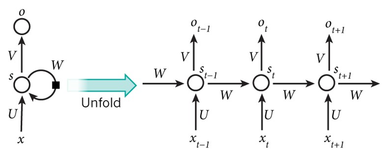
Graph by Nature

Most people think of RNNs in the context of NLP because languages are highly sequential. Indeed, the first RNNs were built for NLP tasks and many nowadays NLP tasks are solved using RNNs. However, they can also be used for tasks dealing with audio, images, videos. For example, you can train an RNN to do the object recognition task on the dataset MNIST, treating each image as a sequence of pixels.

Back-propagation through Time (BPTT)

In a feed forward or a convolutional neural network, errors are back-propagated from the loss to all the layers. These errors are used to update the parameters (weights, biases) according to the update rule that we specify (gradient descent, Adam, ...) to decrease the loss.

In a recurrent neural network, errors are back-propagated from the loss to all the timesteps. The two main differences are:

1. Each layer in a feed-forward network has its own parameters while all the timesteps in a RNN share the same parameters. We use the sum of the gradients at all the timesteps to update the parameters for each training sample/batch.
2. A feed-forward network has a fixed number of layers, while a RNN can have an arbitrary number of timesteps depending on the length of the sequence.

For the number 2, this means that if your sequence is long (say, 1000 steps corresponding to 1000 words in a text document), the process of back-propagating through all those steps is computationally expensive. Another problem is that this can lead to the gradients to be exponentially increasing or decreasing, depending on whether they are big or small, which lead to vanishing or exploding gradients. Denny Britz has a great blog post on the BPTT and exploding/vanishing gradients.

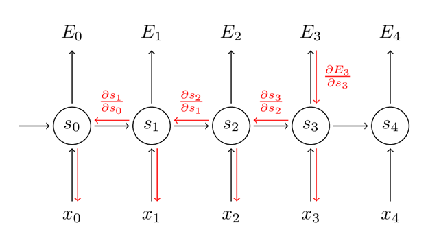
Graph by Denny Britz

To avoid having to do the full parameter update for all the timesteps, we often limit the number of timesteps, resulting in what is known as truncated BPTT. This speeds up computation at each update. The downside is that we can only back-propagate the errors back to a limited number of timesteps, and the network won't be able to learn the dependencies from the beginning of time (e.g., from the beginning of a text).

In TensorFlow, RNNs are created using the unrolled version of the network. In the non-eager mode of TensorFlow, this means that a fixed number of timesteps are specified before executing the computation, and it can only handle input with those exact number of timesteps. This can be problematic since we don't usually have inputs of the exact same length. For example, one paragraph might have 20 words while another might have 200. A common practice is to divide the data into different buckets, with samples of similar lengths into the same bucket. All samples in one bucket will either be padded with zero tokens or truncated to have the same length.

Gated Recurrent Unit (LSTM and GRU)

In practice, RNNs have proven to be really bad at capturing long-term dependencies.To address this drawback, people have been using Long Short-Term Memory (LSTM). The rise of LSTM in the last 3 years makes it seem like a new idea, but it's actually a pretty old concept. It was proposed in the mid-90s by two German researchers, Sepp Hochreiter and Jürgen Schmidhuber, as a solution to the vanishing gradient problem. Like many ideas in AI, LSTM has only become popular in the last few years thanks to the increasing computational power that allows it to work.

Google Trend, Feb 19, 2018

LSTM units use what's called a gating mechanism. They include 4 gates, generally denoted as i, o, f, and c˜, corresponding to input, output, forget, and candidate/new memory gate.

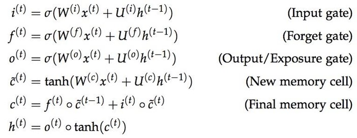
It seems like everyone in academia has a different diagram to visualize the LSTM units, all are inevitably confusing. One of the diagrams that I find less confusing is the one created by Mohammadi et al. for CS224D's lecture note.

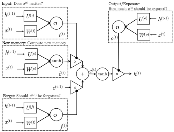
Intuitively, we can think of the gate as controlling what information to enter and emit from the cell at each timestep. All the gates have the same dimensions.

• input gate: decides how much of the current input to let through.
• forget gate: defines how much of the previous state to take into account.
• output gate: defines how much of the hidden state to expose to the next timestep.
• candidate gate: similar to the original RNN, this gate computes the candidate hidden state based on the previous hidden state and the current input.
• final memory cell: the internal memory of the unit combines the candidate hidden state with the input/forget gate information. Final memory cell is then computed with the output gate to decide how much of the final memory cell is to be output as the hidden state for this current step.

LSTM is not the only gating mechanism aimed at improving capturing long term dependencies of RNNs. GRU (gated recurrent unit) uses similar mechanism with significant simplication. It combines LSTM's forget and input gates into a single "update gate." It also merges the candidate/new cell state and the hidden state. The resulting GRU is much simpler than the standard LSTM, while its performances have been shown to be on par with that of LSTM on several benchmark tasks. The simplicity of GRU also means that it requires less computation, which, in theory, should reduce computation time. However, as far as I know, there hasn't been observation of significant improvement in runtime of GRU compared to LSTM.

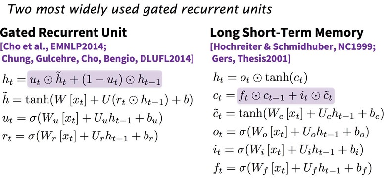
CS224D's lecture note

In TensorFlow, I prefer using GRU as it's a lot less cumbersome. GRU cells in TensorFlow output a hidden state for each layer, while LSTM cells output both candidate and hidden state.

Application: Language modeling

Given a sequence of words we want to predict the distribution of the next word given the all previous words. This ability to predict the next word gives us a generative model that allows us to generate new text by sampling from the output probabilities. Depending on what our training data is, we can generate all kinds of stuff. You can read Andrej Karpathy's blog post about some of the funky results he got using a char-RNN, which is RNNs applied at character- instead of word-level.

When building a language model, our input is typically a sequence of words (or characters, as in the case with char-RNN, or something in between like subwords), and our output is the distribution for the next word.

In this exercise, we will build one char-RNN model on two datasets: Donald Trump's tweets and arvix abstracts. The arvix abstracts dataset consists of 20,466 unique abstracts, most in the range 500 - 2000 characters. The Donald Trump's tweets dataset consists of all his tweets up until Feb 15, 2018, with most of the retweets filtered out. There are 19,469 tweets in total, each of less than 140 characters. We did some minor data-preprocessing: replacing all URL with __HTTP__ (on hindsight, I should have used a shorter token, such as _URL_ or just _U_) and adding end token _E_.

Below are some of the outputs from our presidential tweet bot.

I will be interviewed on @foxandfriends tonight at 10:00 P.M. and the #1 to construct the @WhiteHouse tonight at 10:00 P.M. Enjoy __HTTP__

I will be interviewed on @foxandfriends at 7:00 A.M. and the only one that we will MAKE AMERICA GREAT AGAIN #Trump2016 __HTTP__ __HTTP__

No matter the truth and the world that the Fake News Media will be a great new book #Trump2016 __HTTP__ __HTTP__

Great poll thank you for your support of Monday at 7:30 A.M. on NBC at 7pm #Trump2016 #MakeAmericaGreatAgain #Trump2016 __HTTP__ __HTTP__

The Senate report to our country is a total disaster. The American people who want to start like a total disaster. The American should be the security 5 star with a record contract to the American peop

.@BarackObama is a great president of the @ApprenticeNBC

No matter how the U.S. is a complete the ObamaCare website is a disaster.

Here's an abstract generated by our arvix abstract bot.

"Deep learning neural network architectures can be used to best developing a new architectures contros of the training and max model parametrinal Networks (RNNs) outperform deep learning algorithm is easy to out unclears and can be used to train samples on the state-of-the-art RNN more effective Lorred can be used to best developing a new architectures contros of the training and max model and state-of-the-art deep learning algorithms to a similar pooling relevants. The space of a parameter to optimized hierarchy the state-of-the-art deep learning algorithms to a simple analytical pooling relevants. The space of algorithm is easy to outions of the network are allowed at training and many dectional representations are allow develop a groppose a network by a simple model interact that training algorithms to be the activities to maximul setting, …"

For the code, please see on the class's GitHub. You can also refer to the lecture slides for more information on the code.