梯度下降法实现对数几率回归

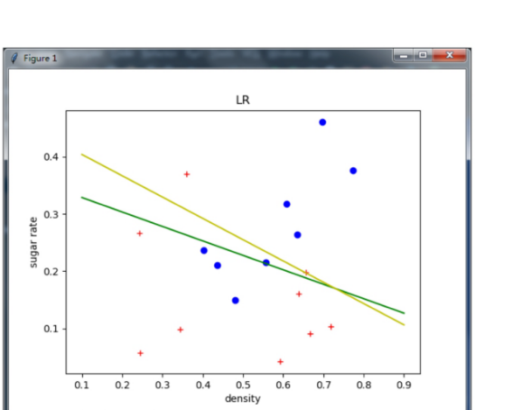
import matplotlib.pyplot as plt
import numpy as np
import xlrd

def sigmoid(x):
    """
    Sigmoid function.
    Input:
        x:np.array
    Return:
        y: the same shape with x
    """    
    y =1.0 / ( 1 + np.exp(-x))
    return y

def newton(X, y):
    """
    Input:
        X: np.array with shape [N, 3]. Input. 
        y: np.array with shape [N, 1]. Label.
    Return:
        beta: np.array with shape [1, 3]. Optimal params with newton method
    """
    N = X.shape[0]
    #initialization
    beta = np.ones((1, 3)) 
    #shape [N, 1]
    z = X.dot(beta.T)
    #log-likehood
    old_l = 0
    new_l = np.sum(-y*z + np.log( 1+np.exp(z) ) )
    iters = 0
    while( np.abs(old_l-new_l) > 1e-5):
        #shape [N, 1]
        p1 = np.exp(z) / (1 + np.exp(z))
        #shape [N, N]
        p = np.diag((p1 * (1-p1)).reshape(N))
        #shape [1, 3]
        first_order = -np.sum(X * (y - p1), 0, keepdims=True)
        #shape [3, 3]
        second_order = X.T .dot(p).dot(X)

        #update
        beta -= first_order.dot(np.linalg.inv(second_order))
        z = X.dot(beta.T)
        old_l = new_l
        new_l = np.sum(-y*z + np.log( 1+np.exp(z) ) )

        iters += 1
    print "iters: ", iters
    print new_l 
    return beta

def gradDescent(X, y):
    """
    Input:
        X: np.array with shape [N, 3]. Input. 
        y: np.array with shape [N, 1]. Label.
    Return:
        beta: np.array with shape [1, 3]. Optimal params with gradient descent method
    """

    N = X.shape[0]
    lr = 0.05
    #initialization
    beta = np.ones((1, 3)) * 0.1
    #shape [N, 1]
    z = X.dot(beta.T)

    for i in range(150):
        #shape [N, 1]
        p1 = np.exp(z) / (1 + np.exp(z))
        #shape [N, N]
        p = np.diag((p1 * (1-p1)).reshape(N))
        #shape [1, 3]
        first_order = -np.sum(X * (y - p1), 0, keepdims=True)

        #update
        beta -= first_order * lr
        z = X.dot(beta.T)

    l = np.sum(-y*z + np.log( 1+np.exp(z) ) )
    print l 
    return beta

if __name__=="__main__":

    #read data from xlsx file
    workbook = xlrd.open_workbook("3.0alpha.xlsx")
    sheet = workbook.sheet_by_name("Sheet1")
    X1 = np.array(sheet.row_values(0))
    X2 = np.array(sheet.row_values(1))
    #this is the extension of x
    X3 = np.array(sheet.row_values(2)) 
    y = np.array(sheet.row_values(3))
    X = np.vstack([X1, X2, X3]).T
    y = y.reshape(-1, 1)

    #plot training data
    for i in range(X1.shape[0]):
        if y[i, 0] == 0:           
            plt.plot(X1[i], X2[i], 'r+')

        else:
            plt.plot(X1[i], X2[i], 'bo')

    #get optimal params beta with newton method 
    beta = newton(X, y)
    newton_left = -( beta[0, 0]*0.1 + beta[0, 2] ) / beta[0, 1]
    newton_right = -( beta[0, 0]*0.9 + beta[0, 2] ) / beta[0, 1]
    plt.plot([0.1, 0.9], [newton_left, newton_right], 'g-')

    #get optimal params beta with gradient descent method
    beta = gradDescent(X, y)
    grad_descent_left = -( beta[0, 0]*0.1 + beta[0, 2] ) / beta[0, 1]
    grad_descent_right = -( beta[0, 0]*0.9 + beta[0, 2] ) / beta[0, 1]
    plt.plot([0.1, 0.9], [grad_descent_left, grad_descent_right], 'y-')

    plt.xlabel('density')
    plt.ylabel('sugar rate')
    plt.title("LR")
    plt.show()