使用一种固定窗函数法设计带通滤波器。
代码:
%% ++++++++++++++++++++++++++++++++++++++++++++++++++++++++++++++++++++++++++++++++
%% Output Info about this m-file
fprintf('
***********************************************************
');
fprintf(' <DSP using MATLAB> Problem 7.16
');
banner();
%% ++++++++++++++++++++++++++++++++++++++++++++++++++++++++++++++++++++++++++++++++
% bandpass
ws1 = 0.3*pi; wp1 = 0.4*pi; wp2 = 0.5*pi; ws2 = 0.6*pi; As = 40; Rp = 0.5;
tr_width = min((wp1-ws1), (ws2-wp2));
[delta1_ori, delta2_ori] = db2delta(Rp, As)
%% ---------------------------------------------------
%% 1 Rectangular Window
%% ---------------------------------------------------
M = ceil(1.8*pi/tr_width) + 1; % Rectangular Window
fprintf('
#1.Rectangular Window, Filter Length M=%d.
', M);
n = [0:1:M-1]; wc1 = (ws1+wp1)/2; wc2 = (wp2+ws2)/2;
hd = ideal_lp(wc2, M) - ideal_lp(wc1, M);
w_rect = (boxcar(M))'; h = hd .* w_rect;
[db, mag, pha, grd, w] = freqz_m(h, [1]); delta_w = 2*pi/1000;
[Hr,ww,P,L] = ampl_res(h);
Rp = -(min(db(wp1/delta_w+1 :1: floor(wp2/delta_w)+1))); % Actual Passband Ripple
fprintf('
Actual Passband Ripple is %.4f dB.
', Rp);
As = -round(max(db(ws2/delta_w+1 : 1 : 501))); % Min Stopband attenuation
fprintf('
Min Stopband attenuation is %.4f dB.
', As);
[delta1_rect, delta2_rect] = db2delta(Rp, As)
%% ----------------------------
%% Plot
%% -----------------------------
figure('NumberTitle', 'off', 'Name', 'Problem 7.16.1 ideal_lp Method')
set(gcf,'Color','white');
subplot(2,2,1); stem(n, hd); axis([0 M-1 -0.3 0.3]); grid on;
xlabel('n'); ylabel('hd(n)'); title('Ideal Impulse Response');
subplot(2,2,2); stem(n, w_rect); axis([0 M-1 0 1.1]); grid on;
xlabel('n'); ylabel('w(n)'); title('Rectangular Window, M=19');
subplot(2,2,3); stem(n, h); axis([0 M-1 -0.3 0.3]); grid on;
xlabel('n'); ylabel('h(n)'); title('Actual Impulse Response');
subplot(2,2,4); plot(w/pi, db); axis([0 1 -100 10]); grid on;
set(gca,'YTickMode','manual','YTick',[-90,-26,0]);
set(gca,'YTickLabelMode','manual','YTickLabel',['90';'26';' 0']);
set(gca,'XTickMode','manual','XTick',[0,0.3,0.4,0.5,0.6,1]);
xlabel('frequency in pi units'); ylabel('Decibels'); title('Magnitude Response in dB');
figure('NumberTitle', 'off', 'Name', 'Problem 7.16.1 h(n) ideal_lp Method')
set(gcf,'Color','white');
subplot(2,2,1); plot(w/pi, db); grid on; %axis([0 1 -100 10]);
xlabel('frequency in pi units'); ylabel('Decibels'); title('Magnitude Response in dB');
set(gca,'YTickMode','manual','YTick',[-90,-26,0])
set(gca,'YTickLabelMode','manual','YTickLabel',['90';'26';' 0']);
set(gca,'XTickMode','manual','XTick',[0,0.3,0.4,0.5,0.6,1,1.4,1.5,1.6,1.7,2]);
subplot(2,2,3); plot(w/pi, mag); grid on; %axis([0 1 -100 10]);
xlabel('frequency in pi units'); ylabel('Absolute'); title('Magnitude Response in absolute');
set(gca,'XTickMode','manual','XTick',[0,0.3,0.4,0.5,0.6,1,1.4,1.5,1.6,1.7,2]);
set(gca,'YTickMode','manual','YTick',[0.0,0.5,1.0])
subplot(2,2,2); plot(w/pi, pha); grid on; %axis([0 1 -100 10]);
xlabel('frequency in pi units'); ylabel('Rad'); title('Phase Response in Radians');
subplot(2,2,4); plot(w/pi, grd*pi/180); grid on; %axis([0 1 -100 10]);
xlabel('frequency in pi units'); ylabel('Rad'); title('Group Delay');
figure('NumberTitle', 'off', 'Name', 'Problem 7.16.1 h(n)')
set(gcf,'Color','white');
plot(ww/pi, Hr); grid on; %axis([0 1 -100 10]);
xlabel('frequency in pi units'); ylabel('Hr'); title('Amplitude Response');
set(gca,'YTickMode','manual','YTick',[-delta2_rect,0,delta2_rect,1 - delta1_rect,1, 1 + delta1_rect])
%% ---------------------------------------------------
%% 2 Bartlett Window
%% ---------------------------------------------------
M = ceil(6.1*pi/tr_width) + 1; % Bartlett Window
fprintf('
#2.Bartlett Window, Filter Length M=%d.
', M);
n = [0:1:M-1]; wc1 = (ws1+wp1)/2; wc2 = (wp2+ws2)/2;
%wc = (ws + wp)/2, % ideal LPF cutoff frequency
hd = ideal_lp(wc2, M) - ideal_lp(wc1, M);
w_bart = (bartlett(M))'; h = hd .* w_bart;
[db, mag, pha, grd, w] = freqz_m(h, [1]); delta_w = 2*pi/1000;
[Hr,ww,P,L] = ampl_res(h);
Rp = -(min(db(wp1/delta_w+1 :1: floor(wp2/delta_w)+1))); % Actual Passband Ripple
fprintf('
Actual Passband Ripple is %.4f dB.
', Rp);
As = -round(max(db(ws2/delta_w+1 : 1 : 501))); % Min Stopband attenuation
fprintf('
Min Stopband attenuation is %.4f dB.
', As);
[delta1_bart, delta2_bart] = db2delta(Rp, As)
%% --------------------------
%% Plot
%% --------------------------
figure('NumberTitle', 'off', 'Name', 'Problem 7.16.2 ideal_lp Method')
set(gcf,'Color','white');
subplot(2,2,1); stem(n, hd); axis([0 M-1 -0.2 0.2]); grid on;
xlabel('n'); ylabel('hd(n)'); title('Ideal Impulse Response');
subplot(2,2,2); stem(n, w_bart); axis([0 M-1 0 1.1]); grid on;
xlabel('n'); ylabel('w(n)'); title('Bartlett Window, M=62');
subplot(2,2,3); stem(n, h); axis([0 M-1 -0.2 0.2]); grid on;
xlabel('n'); ylabel('h(n)'); title('Actual Impulse Response');
subplot(2,2,4); plot(w/pi, db); axis([0 1 -100 10]); grid on;
set(gca,'YTickMode','manual','YTick',[-90,-27,0]);
set(gca,'YTickLabelMode','manual','YTickLabel',['90';'27';' 0']);
set(gca,'XTickMode','manual','XTick',[0,0.3,0.4,0.5,0.6,1]);
xlabel('frequency in pi units'); ylabel('Decibels'); title('Magnitude Response in dB');
figure('NumberTitle', 'off', 'Name', 'Problem 7.16.2 h(n) ideal_lp Method')
set(gcf,'Color','white');
subplot(2,2,1); plot(w/pi, db); grid on; axis([0 2 -100 10]);
xlabel('frequency in pi units'); ylabel('Decibels'); title('Magnitude Response in dB');
set(gca,'YTickMode','manual','YTick',[-90,-27,0])
set(gca,'YTickLabelMode','manual','YTickLabel',['90';'27';' 0']);
set(gca,'XTickMode','manual','XTick',[0,0.3,0.4,0.5,0.6,1,1.4,1.5,1.6,1.7,2]);
subplot(2,2,3); plot(w/pi, mag); grid on; %axis([0 2 -100 10]);
xlabel('frequency in pi units'); ylabel('Absolute'); title('Magnitude Response in absolute');
set(gca,'XTickMode','manual','XTick',[0,0.3,0.4,0.5,0.6,1,1.4,1.5,1.6,1.7,2]);
set(gca,'YTickMode','manual','YTick',[0.0,0.5,1.0])
subplot(2,2,2); plot(w/pi, pha); grid on; %axis([0 1 -100 10]);
xlabel('frequency in pi units'); ylabel('Rad'); title('Phase Response in Radians');
subplot(2,2,4); plot(w/pi, grd*pi/180); grid on; %axis([0 1 -100 10]);
xlabel('frequency in pi units'); ylabel('Rad'); title('Group Delay');
figure('NumberTitle', 'off', 'Name', 'Problem 7.16.2 h(n)')
set(gcf,'Color','white');
plot(ww/pi, Hr); grid on; %axis([0 1 -100 10]);
xlabel('frequency in pi units'); ylabel('Hr'); title('Amplitude Response');
set(gca,'YTickMode','manual','YTick',[-delta2_bart,0,delta2_bart,1-delta1_bart,1, 1+delta1_bart])
%% ---------------------------------------------------
%% 3 Hann Window
%% ---------------------------------------------------
M = ceil(6.2*pi/tr_width) + 1; % Hann Window
fprintf('
#3.Hann Window, Filter Length M=%4d.
', M);
n = [0:1:M-1]; wc1 = (ws1+wp1)/2; wc2 = (wp2+ws2)/2;
%wc = (ws + wp)/2, % ideal LPF cutoff frequency
hd = ideal_lp(wc2, M) - ideal_lp(wc1, M);
w_hann = (hann(M))'; h = hd .* w_hann;
[db, mag, pha, grd, w] = freqz_m(h, [1]); delta_w = 2*pi/1000;
[Hr,ww,P,L] = ampl_res(h);
Rp = -(min(db(wp1/delta_w+1 :1: floor(wp2/delta_w)+1))); % Actual Passband Ripple
fprintf('
Actual Passband Ripple is %.4f dB.
', Rp);
As = -round(max(db(ws2/delta_w+1 : 1 : 501))); % Min Stopband attenuation
fprintf('
Min Stopband attenuation is %.4f dB.
', As);
[delta1_hann, delta2_hann] = db2delta(Rp, As)
%% --------------------------
%% Plot
%% --------------------------
figure('NumberTitle', 'off', 'Name', 'Problem 7.16.3 ideal_lp Method')
set(gcf,'Color','white');
subplot(2,2,1); stem(n, hd); axis([0 M-1 -0.2 0.3]); grid on;
xlabel('n'); ylabel('hd(n)'); title('Ideal Impulse Response');
subplot(2,2,2); stem(n, w_hann); axis([0 M-1 0 1.1]); grid on;
xlabel('n'); ylabel('w(n)'); title('Hann Window, M=63');
subplot(2,2,3); stem(n, h); axis([0 M-1 -0.2 0.3]); grid on;
xlabel('n'); ylabel('h(n)'); title('Actual Impulse Response');
subplot(2,2,4); plot(w/pi, db); axis([0 1 -100 10]); grid on;
set(gca,'YTickMode','manual','YTick',[-90,-43,0]);
set(gca,'YTickLabelMode','manual','YTickLabel',['90';'43';' 0']);
set(gca,'XTickMode','manual','XTick',[0,0.3,0.4,0.5,0.6,1]);
xlabel('frequency in pi units'); ylabel('Decibels'); title('Magnitude Response in dB');
figure('NumberTitle', 'off', 'Name', 'Problem 7.16.3 h(n) ideal_lp Method')
set(gcf,'Color','white');
subplot(2,2,1); plot(w/pi, db); grid on; axis([0 2 -100 10]);
xlabel('frequency in pi units'); ylabel('Decibels'); title('Magnitude Response in dB');
set(gca,'YTickMode','manual','YTick',[-90,-43,0])
set(gca,'YTickLabelMode','manual','YTickLabel',['90';'43';' 0']);
set(gca,'XTickMode','manual','XTick',[0,0.3,0.4,0.5,0.6,1,1.4,1.5,1.6,1.7,2]);
subplot(2,2,3); plot(w/pi, mag); grid on; %axis([0 2 -100 10]);
xlabel('frequency in pi units'); ylabel('Absolute'); title('Magnitude Response in absolute');
set(gca,'XTickMode','manual','XTick',[0,0.3,0.4,0.5,0.6,1,1.4,1.5,1.6,1.7,2]);
set(gca,'YTickMode','manual','YTick',[0.0,0.5,1.0])
subplot(2,2,2); plot(w/pi, pha); grid on; %axis([0 1 -100 10]);
xlabel('frequency in pi units'); ylabel('Rad'); title('Phase Response in Radians');
subplot(2,2,4); plot(w/pi, grd*pi/180); grid on; %axis([0 1 -100 10]);
xlabel('frequency in pi units'); ylabel('Rad'); title('Group Delay');
figure('NumberTitle', 'off', 'Name', 'Problem 7.16.3 h(n)')
set(gcf,'Color','white');
plot(ww/pi, Hr); grid on; %axis([0 1 -100 10]);
xlabel('frequency in pi units'); ylabel('Hr'); title('Amplitude Response');
set(gca,'YTickMode','manual','YTick',[-delta2_hann,0,delta2_hann,1 - delta1_hann,1, 1 + delta1_hann])
%% ---------------------------------------------------
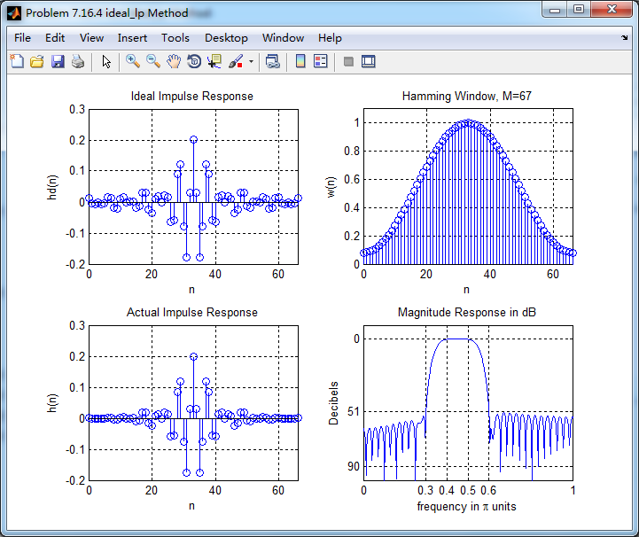
%% 4 Hamming Window
%% ---------------------------------------------------
M = ceil(6.6*pi/tr_width) + 1; % Hamming Window
fprintf('
#4.Hamming Window, Filter Length M=%4d.
', M);
n = [0:1:M-1]; wc1 = (ws1+wp1)/2; wc2 = (wp2+ws2)/2;
%wc = (ws + wp)/2, % ideal LPF cutoff frequency
hd = ideal_lp(wc2, M) - ideal_lp(wc1, M);
w_hamm = (hamming(M))'; h = hd .* w_hamm;
[db, mag, pha, grd, w] = freqz_m(h, [1]); delta_w = 2*pi/1000;
[Hr,ww,P,L] = ampl_res(h);
Rp = -(min(db(wp1/delta_w+1 :1: floor(wp2/delta_w)+1))); % Actual Passband Ripple
fprintf('
Actual Passband Ripple is %.4f dB.
', Rp);
As = -round(max(db(ws2/delta_w+1 : 1 : 501))); % Min Stopband attenuation
fprintf('
Min Stopband attenuation is %.4f dB.
', As);
[delta1_hamm, delta2_hamm] = db2delta(Rp, As)
%% --------------------------
%% Plot
%% --------------------------
figure('NumberTitle', 'off', 'Name', 'Problem 7.16.4 ideal_lp Method')
set(gcf,'Color','white');
subplot(2,2,1); stem(n, hd); axis([0 M-1 -0.2 0.3]); grid on;
xlabel('n'); ylabel('hd(n)'); title('Ideal Impulse Response');
subplot(2,2,2); stem(n, w_hamm); axis([0 M-1 0 1.1]); grid on;
xlabel('n'); ylabel('w(n)'); title('Hamming Window, M=67');
subplot(2,2,3); stem(n, h); axis([0 M-1 -0.2 0.3]); grid on;
xlabel('n'); ylabel('h(n)'); title('Actual Impulse Response');
subplot(2,2,4); plot(w/pi, db); axis([0 1 -100 10]); grid on;
set(gca,'YTickMode','manual','YTick',[-90,-51,0]);
set(gca,'YTickLabelMode','manual','YTickLabel',['90';'51';' 0']);
set(gca,'XTickMode','manual','XTick',[0,0.3,0.4,0.5,0.6,1]);
xlabel('frequency in pi units'); ylabel('Decibels'); title('Magnitude Response in dB');
figure('NumberTitle', 'off', 'Name', 'Problem 7.16.4 h(n) ideal_lp Method')
set(gcf,'Color','white');
subplot(2,2,1); plot(w/pi, db); grid on; axis([0 2 -100 10]);
xlabel('frequency in pi units'); ylabel('Decibels'); title('Magnitude Response in dB');
set(gca,'YTickMode','manual','YTick',[-90,-51,0])
set(gca,'YTickLabelMode','manual','YTickLabel',['90';'51';' 0']);
set(gca,'XTickMode','manual','XTick',[0,0.3,0.4,0.5,0.6,1,1.4,1.5,1.6,1.7,2]);
subplot(2,2,3); plot(w/pi, mag); grid on; %axis([0 2 -100 10]);
xlabel('frequency in pi units'); ylabel('Absolute'); title('Magnitude Response in absolute');
set(gca,'XTickMode','manual','XTick',[0,0.3,0.4,0.5,0.6,1,1.4,1.5,1.6,1.7,2]);
set(gca,'YTickMode','manual','YTick',[0.0,0.5,1.0])
subplot(2,2,2); plot(w/pi, pha); grid on; %axis([0 1 -100 10]);
xlabel('frequency in pi units'); ylabel('Rad'); title('Phase Response in Radians');
subplot(2,2,4); plot(w/pi, grd*pi/180); grid on; %axis([0 1 -100 10]);
xlabel('frequency in pi units'); ylabel('Rad'); title('Group Delay');
figure('NumberTitle', 'off', 'Name', 'Problem 7.16.4 h(n)')
set(gcf,'Color','white');
plot(ww/pi, Hr); grid on; %axis([0 1 -100 10]);
xlabel('frequency in pi units'); ylabel('Hr'); title('Amplitude Response');
set(gca,'YTickMode','manual','YTick',[-delta2_hamm,0,delta2_hamm,1 - delta1_hamm,1, 1 + delta1_hamm])
%% ---------------------------------------------------
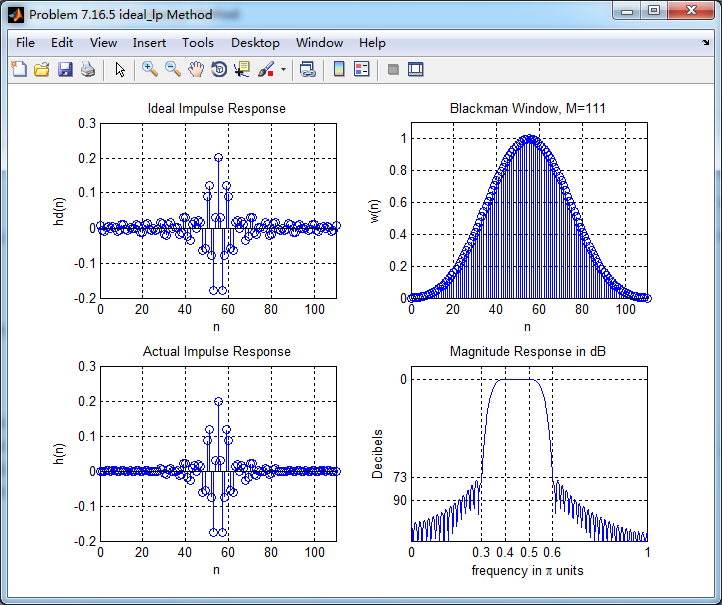
%% 5 Blackman Window
%% ---------------------------------------------------
M = ceil(11*pi/tr_width) + 1; % Blackman Window
fprintf('
#5.Blackman Window, Filter Length M=%d.
', M);
n = [0:1:M-1]; wc1 = (ws1+wp1)/2; wc2 = (wp2+ws2)/2;
%wc = (ws + wp)/2, % ideal LPF cutoff frequency
hd = ideal_lp(wc2, M) - ideal_lp(wc1, M);
w_bla = (blackman(M))'; h = hd .* w_bla;
[db, mag, pha, grd, w] = freqz_m(h, [1]); delta_w = 2*pi/1000;
[Hr,ww,P,L] = ampl_res(h);
Rp = -(min(db(wp1/delta_w+1 :1: floor(wp2/delta_w)+1))); % Actual Passband Ripple
fprintf('
Actual Passband Ripple is %.4f dB.
', Rp);
As = -round(max(db(ws2/delta_w+1 : 1 : 501))); % Min Stopband attenuation
fprintf('
Min Stopband attenuation is %.4f dB.
', As);
[delta1_bla, delta2_bla] = db2delta(Rp, As)
%% --------------------------
%% Plot
%% --------------------------
figure('NumberTitle', 'off', 'Name', 'Problem 7.16.5 ideal_lp Method')
set(gcf,'Color','white');
subplot(2,2,1); stem(n, hd); axis([0 M-1 -0.2 0.3]); grid on;
xlabel('n'); ylabel('hd(n)'); title('Ideal Impulse Response');
subplot(2,2,2); stem(n, w_bla); axis([0 M-1 0 1.1]); grid on;
xlabel('n'); ylabel('w(n)'); title('Blackman Window, M=111');
subplot(2,2,3); stem(n, h); axis([0 M-1 -0.2 0.3]); grid on;
xlabel('n'); ylabel('h(n)'); title('Actual Impulse Response');
subplot(2,2,4); plot(w/pi, db); axis([0 1 -120 10]); grid on;
set(gca,'YTickMode','manual','YTick',[-90,-73,0]);
set(gca,'YTickLabelMode','manual','YTickLabel',['90';'73';' 0']);
set(gca,'XTickMode','manual','XTick',[0,0.3,0.4,0.5,0.6,1]);
xlabel('frequency in pi units'); ylabel('Decibels'); title('Magnitude Response in dB');
figure('NumberTitle', 'off', 'Name', 'Problem 7.16.5 h(n) ideal_lp Method')
set(gcf,'Color','white');
subplot(2,2,1); plot(w/pi, db); grid on; axis([0 2 -120 10]);
xlabel('frequency in pi units'); ylabel('Decibels'); title('Magnitude Response in dB');
set(gca,'YTickMode','manual','YTick',[-90,-73,0])
set(gca,'YTickLabelMode','manual','YTickLabel',['90';'73';' 0']);
set(gca,'XTickMode','manual','XTick',[0,0.3,0.4,0.5,0.6,1,1.4,1.5,1.6,1.7,2]);
subplot(2,2,3); plot(w/pi, mag); grid on; %axis([0 2 -120 10]);
xlabel('frequency in pi units'); ylabel('Absolute'); title('Magnitude Response in absolute');
set(gca,'XTickMode','manual','XTick',[0,0.3,0.4,0.5,0.6,1,1.4,1.5,1.6,1.7,2]);
set(gca,'YTickMode','manual','YTick',[0.0,0.5,1.0])
subplot(2,2,2); plot(w/pi, pha); grid on; %axis([0 1 -100 10]);
xlabel('frequency in pi units'); ylabel('Rad'); title('Phase Response in Radians');
subplot(2,2,4); plot(w/pi, grd*pi/180); grid on; %axis([0 1 -100 10]);
xlabel('frequency in pi units'); ylabel('Rad'); title('Group Delay');
figure('NumberTitle', 'off', 'Name', 'Problem 7.16.5 h(n)')
set(gcf,'Color','white');
plot(ww/pi, Hr); grid on; %axis([0 1 -100 10]);
xlabel('frequency in pi units'); ylabel('Hr'); title('Amplitude Response');
set(gca,'YTickMode','manual','YTick',[-delta2_bla,0,delta2_bla,1-delta1_bla,1, 1+delta1_bla])
%% ---------------------------------------------------
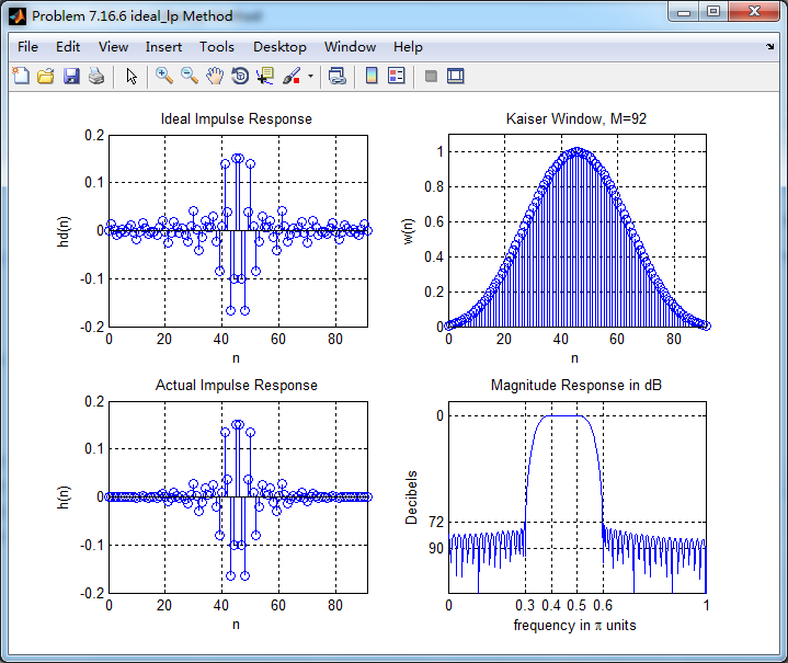
%% 6 Kaiser Window
%% ---------------------------------------------------
M = ceil((As-7.95)/(2.285*tr_width)) + 1; % Kaiser Window
if As > 21 || As < 50
beta = 0.5842*(As-21)^0.4 + 0.07886*(As-21);
else
beta = 0.1102*(As-8.7);
end
fprintf('
#6.Kaiser Window, Filter Length M=%d, beta=%.4f
', M,beta);
n = [0:1:M-1]; wc1 = (ws1+wp1)/2; wc2 = (wp2+ws2)/2;
%wc = (ws + wp)/2, % ideal LPF cutoff frequency
hd = ideal_lp(wc2, M) - ideal_lp(wc1, M);
w_kai = (kaiser(M,beta))'; h = hd .* w_kai;
[db, mag, pha, grd, w] = freqz_m(h, [1]); delta_w = 2*pi/1000;
[Hr,ww,P,L] = ampl_res(h);
Rp = -(min(db(wp1/delta_w+1 :1: floor(wp2/delta_w)+1))); % Actual Passband Ripple
fprintf('
Actual Passband Ripple is %.4f dB.
', Rp);
As = -round(max(db(ws2/delta_w+1 : 1 : 501))); % Min Stopband attenuation
fprintf('
Min Stopband attenuation is %.4f dB.
', As);
[delta1_kai, delta2_kai] = db2delta(Rp, As)
%% --------------------------
%% Plot
%% --------------------------
figure('NumberTitle', 'off', 'Name', 'Problem 7.16.6 ideal_lp Method')
set(gcf,'Color','white');
subplot(2,2,1); stem(n, hd); axis([0 M-1 -0.2 0.2]); grid on;
xlabel('n'); ylabel('hd(n)'); title('Ideal Impulse Response');
subplot(2,2,2); stem(n, w_kai); axis([0 M-1 0 1.1]); grid on;
xlabel('n'); ylabel('w(n)'); title('Kaiser Window, M=92');
subplot(2,2,3); stem(n, h); axis([0 M-1 -0.2 0.2]); grid on;
xlabel('n'); ylabel('h(n)'); title('Actual Impulse Response');
subplot(2,2,4); plot(w/pi, db); axis([0 1 -120 10]); grid on;
set(gca,'YTickMode','manual','YTick',[-90,-72,0]);
set(gca,'YTickLabelMode','manual','YTickLabel',['90';'72';' 0']);
set(gca,'XTickMode','manual','XTick',[0,0.3,0.4,0.5,0.6,1]);
xlabel('frequency in pi units'); ylabel('Decibels'); title('Magnitude Response in dB');
figure('NumberTitle', 'off', 'Name', 'Problem 7.16.6 h(n) ideal_lp Method')
set(gcf,'Color','white');
subplot(2,2,1); plot(w/pi, db); grid on; axis([0 2 -120 10]);
xlabel('frequency in pi units'); ylabel('Decibels'); title('Magnitude Response in dB');
set(gca,'YTickMode','manual','YTick',[-90,-72,0])
set(gca,'YTickLabelMode','manual','YTickLabel',['90';'72';' 0']);
set(gca,'XTickMode','manual','XTick',[0,0.3,0.4,0.5,0.6,1,1.4,1.5,1.6,1.7,2]);
subplot(2,2,3); plot(w/pi, mag); grid on; %axis([0 2 -100 10]);
xlabel('frequency in pi units'); ylabel('Absolute'); title('Magnitude Response in absolute');
set(gca,'XTickMode','manual','XTick',[0,0.3,0.4,0.5,0.6,1,1.4,1.5,1.6,1.7,2]);
set(gca,'YTickMode','manual','YTick',[0.0,0.5,1.0])
subplot(2,2,2); plot(w/pi, pha); grid on; %axis([0 1 -100 10]);
xlabel('frequency in pi units'); ylabel('Rad'); title('Phase Response in Radians');
subplot(2,2,4); plot(w/pi, grd*pi/180); grid on; %axis([0 1 -100 10]);
xlabel('frequency in pi units'); ylabel('Rad'); title('Group Delay');
figure('NumberTitle', 'off', 'Name', 'Problem 7.16.6 h(n)')
set(gcf,'Color','white');
plot(ww/pi, Hr); grid on; %axis([0 1 -100 10]);
xlabel('frequency in pi units'); ylabel('Hr'); title('Amplitude Response');
set(gca,'YTickMode','manual','YTick',[-delta2_kai,0,delta2_kai,1-delta1_kai,1, 1+delta1_kai])
运行结果:
设计指标,As=40dB,Rp=0.5dB;换算成绝对指标,为δ1=0.0288,δ2=0.0103。

由书中表7.1可知,矩形窗(Rectangular)和三角窗(Bartlett)不满足设计要求,这里我们也进行贴图验证。


上图可知,rectangualr窗和bartlett窗不符合设计要求。


下面将以上几种窗函数设计结果,总结如下
| 序号 | 名 称 | 长度M | As | Rp |
| 1 | Rectangular | 19 | 26 | 1.918 |
| 2 | Bartlett | 62 | 27 | 0.1059 |
| 3 | Hann | 63 | 43 | 0.1242 |
| 4 | Hamming | 67 | 51 | 0.0488 |
| 5 | Blackman | 111 | 73 | 0.0027 |
| 6 | Kaiser | 92 | 72 | 0.0049 |
由上表得知,满足设计要求的是用长M=63的Hann窗截断得到的滤波器。