《DSP using MATLAB》Problem 7.34

代码：

%% ++++++++++++++++++++++++++++++++++++++++++++++++++++++++++++++++++++++++++++++++
%%            Output Info about this m-file
fprintf('
***********************************************************
');
fprintf('        <DSP using MATLAB> Problem 7.34 

');

banner();
%% ++++++++++++++++++++++++++++++++++++++++++++++++++++++++++++++++++++++++++++++++

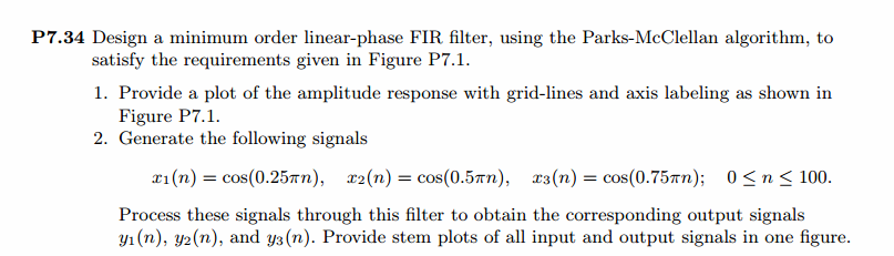
% bandpass in Fig P7.1
ws1 = 0.25*pi; wp1 = 0.35*pi; wp2 = 0.65*pi; ws2=0.75*pi; 
delta1 = 0.05; delta2 = 0.02; delta3 = 0.05;
weights = [1  delta3/delta2  1];

Dw = min((wp1-ws1), (ws2-wp2));
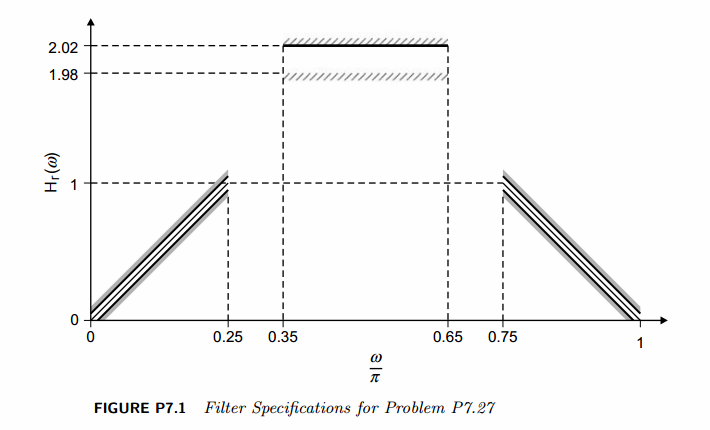
M = ceil((-20*log10((delta1*delta2*delta3)^(1/3)) - 13) / (2.285*Dw) + 1)


deltaH = max([delta1,delta2,delta3]); deltaL = min([delta1,delta2,delta3]);


f = [ 0  ws1 wp1 wp2 ws2  pi]/pi;
m = [ 0  1   2   2   1  0];

h = firpm(M-1, f, m, weights);
[db, mag, pha, grd, w] = freqz_m(h, [1]);
delta_w = 2*pi/1000; 
ws1i = floor(ws1/delta_w)+1; wp1i = floor(wp1/delta_w)+1;
wp2i = floor(wp2/delta_w)+1; ws2i = floor(ws2/delta_w)+1;

Asd = -max(db(1:ws1i))

%[Hr, ww, a, L] = Hr_Type1(h);
[Hr,omega,P,L] = ampl_res(h);
l = 0:M-1;

%% -------------------------------------------------
%%                    Plot
%% -------------------------------------------------  

figure('NumberTitle', 'off', 'Name', 'Problem 7.34 Parks-McClellan Method')
set(gcf,'Color','white'); 

subplot(2,2,1); stem(l, h); axis([-1, M, -0.6, 1.3]); grid on;
xlabel('n'); ylabel('h(n)'); title('Actual Impulse Response, M=23');
set(gca,'XTickMode','manual','XTick',[0,M-1])
set(gca,'YTickMode','manual','YTick',[-0.6:0.2:1.4])

subplot(2,2,2); plot(w/pi, db); axis([0, 1, -80, 10]); grid on;
xlabel('frequency in pi units'); ylabel('Decibels'); title('Magnitude Response in dB ');
set(gca,'XTickMode','manual','XTick',f)
set(gca,'YTickMode','manual','YTick',[-60,-30,0]);
set(gca,'YTickLabelMode','manual','YTickLabel',['60';'30';' 0']);

subplot(2,2,3); plot(omega/pi, Hr); axis([0, 1, -0.2, 2.2]); grid on;
xlabel('frequency in pi nuits'); ylabel('Hr(w)'); title('Amplitude Response');
set(gca,'XTickMode','manual','XTick',f)
set(gca,'YTickMode','manual','YTick',[0,1,1.98,2.02]);

subplot(2,2,4); axis([0, 1, -deltaH, deltaH]); 
sb1w = omega(1:1:ws1i)/pi; sb1e = (Hr(1:1:ws1i)-m(1)); %sb1e = (Hr(1:1:ws1i)-m(1))*weights(1);
pbw = omega(wp1i:wp2i)/pi; pbe = (Hr(wp1i:wp2i)-m(3)); %pbe = (Hr(wp1i:wp2i)-m(3))*weights(2);
sb2w = omega(ws2i:501)/pi; sb2e = (Hr(ws2i:501)-m(5)); %sb2e = (Hr(ws2i:501)-m(5))*weights(3);
plot(sb1w,sb1e,pbw,pbe,sb2w,sb2e); grid on;
xlabel('frequency in pi units'); ylabel('Hr(w)'); title('Error Response'); %title('Weighted Error');
set(gca,'XTickMode','manual','XTick',f);
%set(gca,'YTickMode','manual','YTick',[-deltaH,0,deltaH]);


figure('NumberTitle', 'off', 'Name', 'Problem 7.34 AmpRes of h(n), Parks-McClellan Method')
set(gcf,'Color','white'); 

plot(omega/pi, Hr); grid on; %axis([0 1 -100 10]); 
xlabel('frequency in pi units'); ylabel('Hr'); title('Amplitude Response');
set(gca,'YTickMode','manual','YTick',[0, 1, 1.98, 2.02]);
%set(gca,'YTickLabelMode','manual','YTickLabel',['90';'40';' 0']);
set(gca,'XTickMode','manual','XTick',[0,0.25,0.35,0.65,0.75,1]);

%% -------------------------------------------------------
%%       Input is given, and we want the Output
%% -------------------------------------------------------
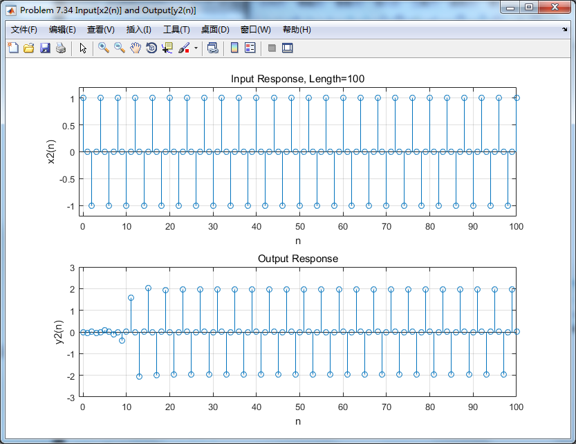
num = 100; 
n_x1 = [0:1:num]; x1 = cos(0.25*pi*n_x1);

n_x2 = n_x1; x2 = cos(0.5*pi*n_x2);

n_x3 = n_x1; x3 = cos(0.75*pi*n_x3);

% Output
y1 = filter(h, 1, x1);
n_y1 = n_x1;

y2 = filter(h, 1, x2);
n_y2 = n_x2;

y3 = filter(h, 1, x3);
n_y3 = n_x3;


figure('NumberTitle', 'off', 'Name', 'Problem 7.34 Input[x1(n)] and Output[y1(n)]');
set(gcf,'Color','white');
subplot(2,1,1); stem(n_x1, x1); axis([-1, 100, -1.2, 1.2]); grid on;
xlabel('n'); ylabel('x1(n)'); title('Input Response, Length=100');
subplot(2,1,2); stem(n_y1, y1); axis([-1, 100, -2, 2]); grid on;
xlabel('n'); ylabel('y1(n)'); title('Output Response');

figure('NumberTitle', 'off', 'Name', 'Problem 7.34 Input[x2(n)] and Output[y2(n)]');
set(gcf,'Color','white');
subplot(2,1,1); stem(n_x2, x2); axis([-1, 100, -1.2, 1.2]); grid on;
xlabel('n'); ylabel('x2(n)'); title('Input Response, Length=100');
subplot(2,1,2); stem(n_y2, y2); axis([-1, 100, -3, 3]); grid on;
xlabel('n'); ylabel('y2(n)'); title('Output Response');

figure('NumberTitle', 'off', 'Name', 'Problem 7.34 Input[x3(n)] and Output[y3(n)]');
set(gcf,'Color','white');
subplot(2,1,1); stem(n_x3, x3); axis([-1, 100, -1.2, 1.2]); grid on;
xlabel('n'); ylabel('x3(n)'); title('Input Response, Length=100');
subplot(2,1,2); stem(n_y3, y3); axis([-1, 100, -2, 2]); grid on;
xlabel('n'); ylabel('y3(n)'); title('Output Response');



% ---------------------------
%    DTFT of x and y
% ---------------------------
MM = 500;
[X1, w1] = dtft1(x1, n_x1, MM);
[Y1, w1] = dtft1(y1, n_y1, MM);
[X2, w1] = dtft1(x2, n_x2, MM);
[Y2, w1] = dtft1(y2, n_y2, MM);
[X3, w1] = dtft1(x3, n_x3, MM);
[Y3, w1] = dtft1(y3, n_y3, MM);

magX1 = abs(X1); angX1 = angle(X1); realX1 = real(X1); imagX1 = imag(X1);
magY1 = abs(Y1); angY1 = angle(Y1); realY1 = real(Y1); imagY1 = imag(Y1);
magX2 = abs(X2); angX2 = angle(X2); realX2 = real(X2); imagX2 = imag(X2);
magY2 = abs(Y2); angY2 = angle(Y2); realY2 = real(Y2); imagY2 = imag(Y2);
magX3 = abs(X3); angX3 = angle(X3); realX3 = real(X3); imagX3 = imag(X3);
magY3 = abs(Y3); angY3 = angle(Y3); realY3 = real(Y3); imagY3 = imag(Y3);

figure('NumberTitle', 'off', 'Name', 'Problem 7.34 DTFT of Input[x1(n)]')
set(gcf,'Color','white'); 
subplot(2,2,1); plot(w1/pi,magX1); grid on; %axis([0,2,0,15]); 
title('Magnitude Part');
xlabel('frequency in pi units'); ylabel('Magnitude  |X|'); 
subplot(2,2,3); plot(w1/pi, angX1/pi); grid on; axis([0,2,-1,1]);
title('Angle Part');
xlabel('frequency in pi units'); ylabel('Radians/pi');

subplot(2,2,2); plot(w1/pi, realX1); grid on;
title('Real Part');
xlabel('frequency in pi units'); ylabel('Real');
subplot(2,2,4); plot(w1/pi, imagX1); grid on;
title('Imaginary Part');
xlabel('frequency in pi units'); ylabel('Imaginary');


figure('NumberTitle', 'off', 'Name', 'Problem 7.34 DTFT of Output[y1(n)]')
set(gcf,'Color','white'); 
subplot(2,2,1); plot(w1/pi,magY1); grid on; %axis([0,2,0,15]); 
title('Magnitude Part');
xlabel('frequency in pi units'); ylabel('Magnitude  |Y|'); 
subplot(2,2,3); plot(w1/pi, angY1/pi); grid on; axis([0,2,-1,1]);
title('Angle Part');
xlabel('frequency in pi units'); ylabel('Radians/pi');

subplot(2,2,2); plot(w1/pi, realY1); grid on;
title('Real Part');
xlabel('frequency in pi units'); ylabel('Real');
subplot(2,2,4); plot(w1/pi, imagY1); grid on;
title('Imaginary Part');
xlabel('frequency in pi units'); ylabel('Imaginary');

figure('NumberTitle', 'off', 'Name', 'Problem 7.34 Magnitude Response')
set(gcf,'Color','white'); 
subplot(1,2,1); plot(w1/pi,magX1); grid on; %axis([0,2,0,15]); 
title('Magnitude Part of Input');
xlabel('frequency in pi units'); ylabel('Magnitude  |X|'); 
subplot(1,2,2); plot(w1/pi,magY1); grid on; %axis([0,2,0,15]); 
title('Magnitude Part of Output');
xlabel('frequency in pi units'); ylabel('Magnitude  |Y|'); 





figure('NumberTitle', 'off', 'Name', 'Problem 7.34 DTFT of Input[x2(n)]')
set(gcf,'Color','white'); 
subplot(2,2,1); plot(w1/pi,magX2); grid on; %axis([0,2,0,15]); 
title('Magnitude Part');
xlabel('frequency in pi units'); ylabel('Magnitude  |X|'); 
subplot(2,2,3); plot(w1/pi, angX2/pi); grid on; axis([0,2,-1,1]);
title('Angle Part');
xlabel('frequency in pi units'); ylabel('Radians/pi');

subplot(2,2,2); plot(w1/pi, realX2); grid on;
title('Real Part');
xlabel('frequency in pi units'); ylabel('Real');
subplot(2,2,4); plot(w1/pi, imagX2); grid on;
title('Imaginary Part');
xlabel('frequency in pi units'); ylabel('Imaginary');


figure('NumberTitle', 'off', 'Name', 'Problem 7.34 DTFT of Output[y2(n)]')
set(gcf,'Color','white'); 
subplot(2,2,1); plot(w1/pi,magY2); grid on; %axis([0,2,0,15]); 
title('Magnitude Part');
xlabel('frequency in pi units'); ylabel('Magnitude  |Y|'); 
subplot(2,2,3); plot(w1/pi, angY2/pi); grid on; axis([0,2,-1,1]);
title('Angle Part');
xlabel('frequency in pi units'); ylabel('Radians/pi');

subplot(2,2,2); plot(w1/pi, realY2); grid on;
title('Real Part');
xlabel('frequency in pi units'); ylabel('Real');
subplot(2,2,4); plot(w1/pi, imagY2); grid on;
title('Imaginary Part');
xlabel('frequency in pi units'); ylabel('Imaginary');

figure('NumberTitle', 'off', 'Name', 'Problem 7.34 Magnitude Response')
set(gcf,'Color','white'); 
subplot(1,2,1); plot(w1/pi,magX2); grid on; %axis([0,2,0,15]); 
title('Magnitude Part of Input');
xlabel('frequency in pi units'); ylabel('Magnitude  |X|'); 
subplot(1,2,2); plot(w1/pi,magY2); grid on; %axis([0,2,0,15]); 
title('Magnitude Part of Output');
xlabel('frequency in pi units'); ylabel('Magnitude  |Y|'); 





figure('NumberTitle', 'off', 'Name', 'Problem 7.34 DTFT of Input[x3(n)]')
set(gcf,'Color','white'); 
subplot(2,2,1); plot(w1/pi,magX3); grid on; %axis([0,2,0,15]); 
title('Magnitude Part');
xlabel('frequency in pi units'); ylabel('Magnitude  |X|'); 
subplot(2,2,3); plot(w1/pi, angX3/pi); grid on; axis([0,2,-1,1]);
title('Angle Part');
xlabel('frequency in pi units'); ylabel('Radians/pi');

subplot(2,2,2); plot(w1/pi, realX3); grid on;
title('Real Part');
xlabel('frequency in pi units'); ylabel('Real');
subplot(2,2,4); plot(w1/pi, imagX3); grid on;
title('Imaginary Part');
xlabel('frequency in pi units'); ylabel('Imaginary');


figure('NumberTitle', 'off', 'Name', 'Problem 7.34 DTFT of Output[y3(n)]')
set(gcf,'Color','white'); 
subplot(2,2,1); plot(w1/pi,magY3); grid on; %axis([0,2,0,15]); 
title('Magnitude Part');
xlabel('frequency in pi units'); ylabel('Magnitude  |Y|'); 
subplot(2,2,3); plot(w1/pi, angY3/pi); grid on; axis([0,2,-1,1]);
title('Angle Part');
xlabel('frequency in pi units'); ylabel('Radians/pi');

subplot(2,2,2); plot(w1/pi, realY3); grid on;
title('Real Part');
xlabel('frequency in pi units'); ylabel('Real');
subplot(2,2,4); plot(w1/pi, imagY3); grid on;
title('Imaginary Part');
xlabel('frequency in pi units'); ylabel('Imaginary');

figure('NumberTitle', 'off', 'Name', 'Problem 7.34 Magnitude Response')
set(gcf,'Color','white'); 
subplot(1,2,1); plot(w1/pi,magX3); grid on; %axis([0,2,0,15]); 
title('Magnitude Part of Input');
xlabel('frequency in pi units'); ylabel('Magnitude  |X|'); 
subplot(1,2,2); plot(w1/pi,magY3); grid on; %axis([0,2,0,15]); 
title('Magnitude Part of Output');
xlabel('frequency in pi units'); ylabel('Magnitude  |Y|'); 

　　运行结果：

       用P-M法设计出来滤波器长度M=23

        幅度谱如下

        振幅谱如下：

        第2个输入，及对应的输出

        第2个输入输出的谱（DTFT）对比：

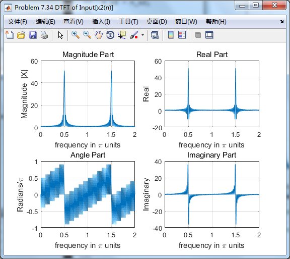
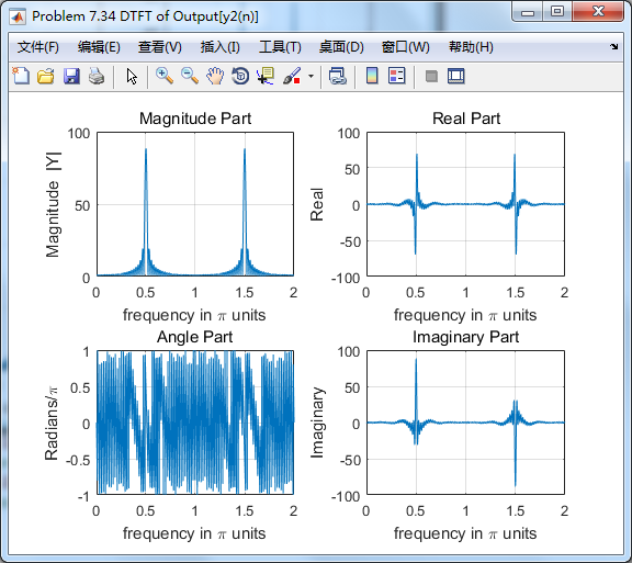
        从图中看，输入0.5π分量幅度有所增大，几乎达到原来的2倍。