《DSP using MATLAB》Problem 8.2

    代码：

%% ------------------------------------------------------------------------
%%            Output Info about this m-file
fprintf('
***********************************************************
');
fprintf('        <DSP using MATLAB> Problem 8.2 

');
banner();
%% ------------------------------------------------------------------------

% digital resonator
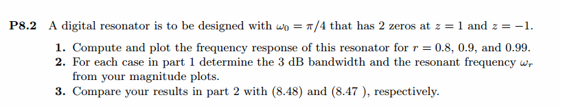
r = 0.8
%r = 0.9
%r = 0.99
omega0 = pi/4;

% corresponding system function  Direct form
%     zeros at z=±1
G = (1-r)*sqrt(1+r*r-2*r*cos(2*omega0)) / sqrt(2*(1-cos(2*omega0)))     % gain parameter
b = G*[1  0  -1];                                                        % denominator                      
a = [1 -2*r*cos(omega0) r*r];                                            % numerator

% precise resonant frequency and 3dB bandwidth
omega_r = acos((1+r*r)*cos(omega0)/(2*r));
delta_omega = 2*(1-r);
fprintf('
Resonant Freq is : %.4fpi unit, 3dB bandwidth is %.4f 
', omega_r/pi,delta_omega);
% 

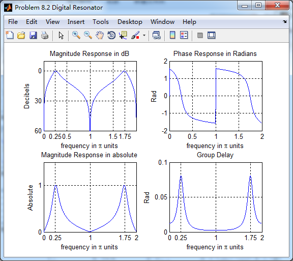
[db, mag, pha, grd, w] = freqz_m(b, a);

figure('NumberTitle', 'off', 'Name', 'Problem 8.2 Digital Resonator')
set(gcf,'Color','white'); 

subplot(2,2,1); plot(w/pi, db); grid on; axis([0 2 -60 10]); 
set(gca,'YTickMode','manual','YTick',[-60,-30,0])
set(gca,'YTickLabelMode','manual','YTickLabel',['60';'30';' 0']);
set(gca,'XTickMode','manual','XTick',[0,0.25,0.5,1,1.5,1.75]);
xlabel('frequency in pi units'); ylabel('Decibels'); title('Magnitude Response in dB');

subplot(2,2,3); plot(w/pi, mag); grid on; %axis([0 1 -100 10]); 
xlabel('frequency in pi units'); ylabel('Absolute'); title('Magnitude Response in absolute');
set(gca,'XTickMode','manual','XTick',[0,0.25,1,1.75,2]);
set(gca,'YTickMode','manual','YTick',[0,1.0]);

subplot(2,2,2); plot(w/pi, pha); grid on; %axis([0 1 -100 10]); 
xlabel('frequency in pi units'); ylabel('Rad'); title('Phase Response in Radians');

subplot(2,2,4); plot(w/pi, grd*pi/180);  grid on; %axis([0 1 -100 10]); 
xlabel('frequency in pi units'); ylabel('Rad'); title('Group Delay');
set(gca,'XTickMode','manual','XTick',[0,0.25,1,1.75,2]);
%set(gca,'YTickMode','manual','YTick',[0,1.0]);

figure('NumberTitle', 'off', 'Name', 'Problem 8.2 Pole-Zero Plot')
set(gcf,'Color','white'); 
zplane(b,a); 
title(sprintf('Pole-Zero Plot, r=%.2f  %.2f\pi',r,omega0/pi));
%pzplotz(b,a);


% Impulse Response
fprintf('
----------------------------------');
fprintf('
Partial fraction expansion method: 
');
[R, p, c] = residuez(b,a)
MR = (abs(R))'              % Residue  Magnitude
AR = (angle(R))'/pi         % Residue  angles in pi units
Mp = (abs(p))'              % pole  Magnitude
Ap = (angle(p))'/pi         % pole  angles in pi units
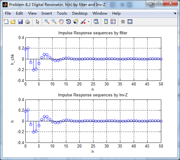
[delta, n] = impseq(0,0,50);
h_chk = filter(b,a,delta);      % check sequences

h =  ( 0.8.^n ) .* (2*0.232*cos(pi*n/4) - 2*0.0509*sin(pi*n/4)) -0.283 * delta;  % r=0.8
%h =  ( 0.9.^n ) .* (2*0.1063*cos(pi*n/4) - 2*0.0112*sin(pi*n/4)) -0.1174 * delta;  % r=0.9
%h =  ( 0.99.^n ) .* (2*0.0101*cos(pi*n/4) - 2*0.0001*sin(pi*n/4)) -0.0102 * delta;  % r=0.99

figure('NumberTitle', 'off', 'Name', 'Problem 8.2 Digital Resonator, h(n) by filter and Inv-Z ')
set(gcf,'Color','white'); 

subplot(2,1,1); stem(n, h_chk); grid on; %axis([0 2 -60 10]); 
xlabel('n'); ylabel('h\_chk'); title('Impulse Response sequences by filter');

subplot(2,1,2); stem(n, h); grid on; %axis([0 1 -100 10]); 
xlabel('n'); ylabel('h'); title('Impulse Response sequences by Inv-Z');


[db, mag, pha, grd, w] = freqz_m(h, [1]);


figure('NumberTitle', 'off', 'Name', 'Problem 8.2 Digital Resonator, h(n) by Inv-Z ')
set(gcf,'Color','white'); 

subplot(2,2,1); plot(w/pi, db); grid on; axis([0 2 -60 10]); 
set(gca,'YTickMode','manual','YTick',[-60,-30,0])
set(gca,'YTickLabelMode','manual','YTickLabel',['60';'30';' 0']);
set(gca,'XTickMode','manual','XTick',[0,0.25,0.5,1,1.5,1.75]);
xlabel('frequency in pi units'); ylabel('Decibels'); title('Magnitude Response in dB');

subplot(2,2,3); plot(w/pi, mag); grid on; %axis([0 1 -100 10]); 
xlabel('frequency in pi units'); ylabel('Absolute'); title('Magnitude Response in absolute');
set(gca,'XTickMode','manual','XTick',[0,0.25,1,1.75,2]);
set(gca,'YTickMode','manual','YTick',[0,1.0]);

subplot(2,2,2); plot(w/pi, pha); grid on; %axis([0 1 -100 10]); 
xlabel('frequency in pi units'); ylabel('Rad'); title('Phase Response in Radians');

subplot(2,2,4); plot(w/pi, grd*pi/180);  grid on; %axis([0 1 -100 10]); 
xlabel('frequency in pi units'); ylabel('Rad'); title('Group Delay');
set(gca,'XTickMode','manual','XTick',[0,0.25,1,1.75,2]);
%set(gca,'YTickMode','manual','YTick',[0,1.0]);

　　运行结果：

       这里的G为增益系数，使得幅度谱在共振频率处最大，等于1

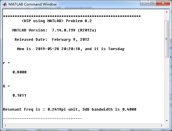
        系统函数部分分式展开

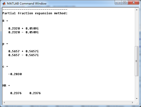
        系统函数的零极点图

        h_chk是由将脉冲序列当成系统输入而得到的，h是由系统函数部分分时展开后查表求逆z变换得到的，

二者幅度谱一致，但是相位谱和群延迟稍有不同。

        r=0.9和0.99的结果这里就不放了。