
代码:
%% ------------------------------------------------------------------------
%% Output Info about this m-file
fprintf('
***********************************************************
');
fprintf(' <DSP using MATLAB> Problem 8.7
');
banner();
%% ------------------------------------------------------------------------
% digital iir lowpass filter
b = [1 1];
a = [1 -0.9];
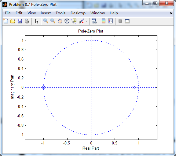
figure('NumberTitle', 'off', 'Name', 'Problem 8.7 Pole-Zero Plot')
set(gcf,'Color','white');
zplane(b,a);
title(sprintf('Pole-Zero Plot'));
%pzplotz(b,a);
% corresponding system function Direct form
K = 1; % gain parameter
b = K*b; % denominator
a = a; % numerator
[db, mag, pha, grd, w] = freqz_m(b, a);
% ---------------------------------------------------------------------
% Choose the gain parameter of the filter, maximum gain is equal to 1
% ---------------------------------------------------------------------
gain1=max(mag) % with poles
K = 1/gain1
[db, mag, pha, grd, w] = freqz_m(K*b, a);
figure('NumberTitle', 'off', 'Name', 'Problem 8.7 IIR lowpass filter')
set(gcf,'Color','white');
subplot(2,2,1); plot(w/pi, db); grid on; axis([0 2 -60 10]);
set(gca,'YTickMode','manual','YTick',[-60,-30,0])
set(gca,'YTickLabelMode','manual','YTickLabel',['60';'30';' 0']);
set(gca,'XTickMode','manual','XTick',[0,0.25,0.5,1,1.5,1.75,2]);
xlabel('frequency in pi units'); ylabel('Decibels'); title('Magnitude Response in dB');
subplot(2,2,3); plot(w/pi, mag); grid on; %axis([0 1 -100 10]);
xlabel('frequency in pi units'); ylabel('Absolute'); title('Magnitude Response in absolute');
set(gca,'XTickMode','manual','XTick',[0,0.25,0.5,1,1.5,1.75,2]);
set(gca,'YTickMode','manual','YTick',[0,1.0]);
subplot(2,2,2); plot(w/pi, pha); grid on; %axis([0 1 -100 10]);
xlabel('frequency in pi units'); ylabel('Rad'); title('Phase Response in Radians');
subplot(2,2,4); plot(w/pi, grd*pi/180); grid on; %axis([0 1 -100 10]);
xlabel('frequency in pi units'); ylabel('Rad'); title('Group Delay');
set(gca,'XTickMode','manual','XTick',[0,0.25,0.5,1,1.5,1.75,2]);
%set(gca,'YTickMode','manual','YTick',[0,1.0]);
% Impulse Response
fprintf('
----------------------------------');
fprintf('
Partial fraction expansion method:
');
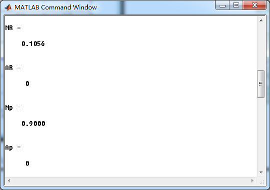
[R, p, c] = residuez(b,a)
MR = (abs(R))' % Residue Magnitude
AR = (angle(R))'/pi % Residue angles in pi units
Mp = (abs(p))' % pole Magnitude
Ap = (angle(p))'/pi % pole angles in pi units
[delta, n] = impseq(0,0,50);
h_chk = filter(b,a,delta); % check sequences
% ------------------------------------------------------------------------------------------------
% gain parameter K=0.05
% ------------------------------------------------------------------------------------------------
h = ( 0.9.^n ) .* 0.1056 - 0.0556 * delta;
% ------------------------------------------------------------------------------------------------
figure('NumberTitle', 'off', 'Name', 'Problem 8.7 IIR lp filter, h(n) by filter and Inv-Z ')
set(gcf,'Color','white');
subplot(2,1,1); stem(n, h_chk); grid on; %axis([0 2 -60 10]);
xlabel('n'); ylabel('h\_chk'); title('Impulse Response sequences by filter');
subplot(2,1,2); stem(n, h); grid on; %axis([0 1 -100 10]);
xlabel('n'); ylabel('h'); title('Impulse Response sequences by Inv-Z');
[db, mag, pha, grd, w] = freqz_m(h, [1]);
figure('NumberTitle', 'off', 'Name', 'Problem 8.7 IIR filter, h(n) by Inv-Z ')
set(gcf,'Color','white');
subplot(2,2,1); plot(w/pi, db); grid on; axis([0 2 -60 10]);
set(gca,'YTickMode','manual','YTick',[-60,-30,0])
set(gca,'YTickLabelMode','manual','YTickLabel',['60';'30';' 0']);
set(gca,'XTickMode','manual','XTick',[0,0.25,1,1.75,2]);
xlabel('frequency in pi units'); ylabel('Decibels'); title('Magnitude Response in dB');
subplot(2,2,3); plot(w/pi, mag); grid on; %axis([0 1 -100 10]);
xlabel('frequency in pi units'); ylabel('Absolute'); title('Magnitude Response in absolute');
set(gca,'XTickMode','manual','XTick',[0,0.25,1,1.75,2]);
set(gca,'YTickMode','manual','YTick',[0,1.0]);
subplot(2,2,2); plot(w/pi, pha); grid on; %axis([0 1 -100 10]);
xlabel('frequency in pi units'); ylabel('Rad'); title('Phase Response in Radians');
subplot(2,2,4); plot(w/pi, grd*pi/180); grid on; %axis([0 1 -100 10]);
xlabel('frequency in pi units'); ylabel('Rad'); title('Group Delay');
set(gca,'XTickMode','manual','XTick',[0,0.25,1,1.75,2]);
%set(gca,'YTickMode','manual','YTick',[0,1.0]);
% --------------------------------------------------
% digital IIR comb filter
% --------------------------------------------------
b = K*[1 0 0 0 0 0 1];
a = [1 0 0 0 0 0 -0.9];
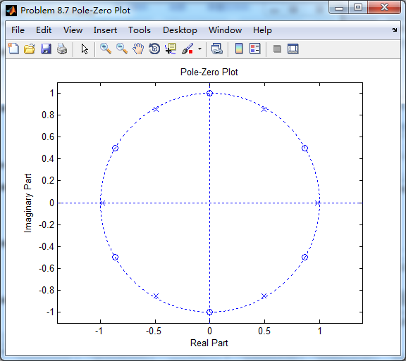
figure('NumberTitle', 'off', 'Name', 'Problem 8.7 Pole-Zero Plot')
set(gcf,'Color','white');
zplane(b,a);
title(sprintf('Pole-Zero Plot'));
[db, mag, pha, grd, w] = freqz_m(b, a);
figure('NumberTitle', 'off', 'Name', 'Problem 8.7 IIR comb filter')
set(gcf,'Color','white');
subplot(2,2,1); plot(w/pi, db); grid on; axis([0 2 -60 10]);
set(gca,'YTickMode','manual','YTick',[-60,-30,0])
set(gca,'YTickLabelMode','manual','YTickLabel',['60';'30';' 0']);
set(gca,'XTickMode','manual','XTick',[0,0.25,0.5,1,1.5,1.75,2]);
xlabel('frequency in pi units'); ylabel('Decibels'); title('Magnitude Response in dB');
subplot(2,2,3); plot(w/pi, mag); grid on; %axis([0 1 -100 10]);
xlabel('frequency in pi units'); ylabel('Absolute'); title('Magnitude Response in absolute');
set(gca,'XTickMode','manual','XTick',[0,0.25,0.5,1,1.5,1.75,2]);
set(gca,'YTickMode','manual','YTick',[0,1.0]);
subplot(2,2,2); plot(w/pi, pha); grid on; %axis([0 1 -100 10]);
xlabel('frequency in pi units'); ylabel('Rad'); title('Phase Response in Radians');
subplot(2,2,4); plot(w/pi, grd*pi/180); grid on; %axis([0 1 -100 10]);
xlabel('frequency in pi units'); ylabel('Rad'); title('Group Delay');
set(gca,'XTickMode','manual','XTick',[0,0.25,0.5,1,1.5,1.75,2]);
%set(gca,'YTickMode','manual','YTick',[0,1.0]);
% Impulse Response
fprintf('
----------------------------------');
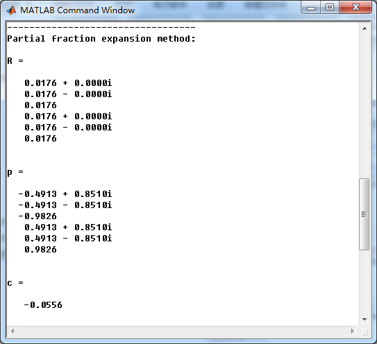
fprintf('
Partial fraction expansion method:
');
[R, p, c] = residuez(b,a)
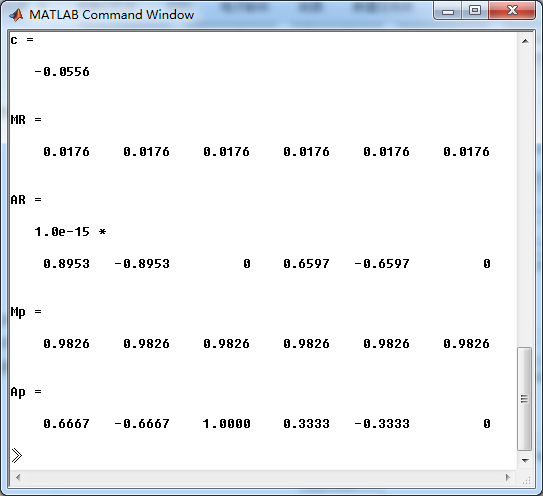
MR = (abs(R))' % Residue Magnitude
AR = (angle(R))'/pi % Residue angles in pi units
Mp = (abs(p))' % pole Magnitude
Ap = (angle(p))'/pi % pole angles in pi units
[delta, n] = impseq(0,0,300);
h_chk = filter(b,a,delta); % check sequences
% ------------------------------------------------------------------------------------------------
% gain parameter K=0.05
% ------------------------------------------------------------------------------------------------
%h = 0.0211 * (( 0.9791.^n ) .* (2*cos(0.4*pi*n) + 2*cos(0.8*pi*n) + 1)) - 0.0556*delta; %L=5;
h = 0.0176 * ( ( 0.9826.^n ) .* ( 2*cos(2*pi*n/3) + 2*cos(pi*n/3) + (-1).^n + 1) ) - 0.0556*delta; %L=6;
% ------------------------------------------------------------------------------------------------
figure('NumberTitle', 'off', 'Name', 'Problem 8.7 Comb filter, h(n) by filter and Inv-Z ')
set(gcf,'Color','white');
subplot(2,1,1); stem(n, h_chk); grid on; %axis([0 2 -60 10]);
xlabel('n'); ylabel('h\_chk'); title('Impulse Response sequences by filter');
subplot(2,1,2); stem(n, h); grid on; %axis([0 1 -100 10]);
xlabel('n'); ylabel('h'); title('Impulse Response sequences by Inv-Z');
[db, mag, pha, grd, w] = freqz_m(h, [1]);
figure('NumberTitle', 'off', 'Name', 'Problem 8.7 Comb filter, h(n) by Inv-Z ')
set(gcf,'Color','white');
subplot(2,2,1); plot(w/pi, db); grid on; axis([0 2 -60 10]);
set(gca,'YTickMode','manual','YTick',[-60,-30,0])
set(gca,'YTickLabelMode','manual','YTickLabel',['60';'30';' 0']);
set(gca,'XTickMode','manual','XTick',[0,0.25,1,1.75,2]);
xlabel('frequency in pi units'); ylabel('Decibels'); title('Magnitude Response in dB');
subplot(2,2,3); plot(w/pi, mag); grid on; %axis([0 1 -100 10]);
xlabel('frequency in pi units'); ylabel('Absolute'); title('Magnitude Response in absolute');
set(gca,'XTickMode','manual','XTick',[0,0.25,1,1.75,2]);
set(gca,'YTickMode','manual','YTick',[0,1.0]);
subplot(2,2,2); plot(w/pi, pha); grid on; %axis([0 1 -100 10]);
xlabel('frequency in pi units'); ylabel('Rad'); title('Phase Response in Radians');
subplot(2,2,4); plot(w/pi, grd*pi/180); grid on; %axis([0 1 -100 10]);
xlabel('frequency in pi units'); ylabel('Rad'); title('Group Delay');
set(gca,'XTickMode','manual','XTick',[0,0.25,1,1.75,2]);
%set(gca,'YTickMode','manual','YTick',[0,1.0]);
运行结果:
先计算单个IIR低通,

零极点

L=6阶梳状低通,系统函数部分分式展开如下
梳状低通滤波器零极点图
幅度谱、相位谱、群延迟
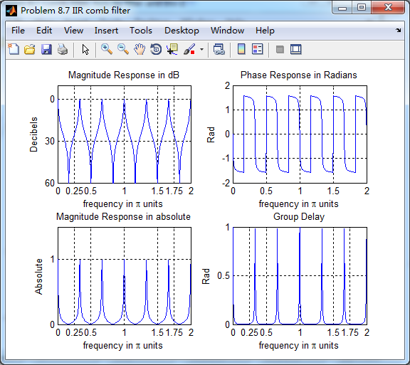
可以看出,在0到2π范围内,单个低通重复出现了6次,原来的谱压缩到六分之一。