代码:
%% ------------------------------------------------------------------------
%% Output Info about this m-file
fprintf('
***********************************************************
');
fprintf(' <DSP using MATLAB> Problem 8.33.2
');
banner();
%% ------------------------------------------------------------------------
% Digital Filter Specifications:
wp = 0.45*pi; % digital passband freq in rad
ws = 0.50*pi; % digital stopband freq in rad
Rp = 0.5; % passband ripple in dB
As = 60; % stopband attenuation in dB
Ripple = 10 ^ (-Rp/20) % passband ripple in absolute
Attn = 10 ^ (-As/20) % stopband attenuation in absolute
% Analog prototype specifications: Inverse Mapping for frequencies
T = 1; % set T = 1
Fs = 1/T;
OmegaP = (2/T)*tan(wp/2); % Prewarp(Cutoff) prototype passband freq
OmegaS = (2/T)*tan(ws/2); % Prewarp(cutoff) prototype stopband freq
OmegaP/pi
OmegaS/pi
% ---------------------------------------------------------------
% method 1: afd_chb1 function
% ---------------------------------------------------------------
% Analog Chebyshev-1 Prototype Filter Calculation:
[cs, ds] = afd_chb1(OmegaP, OmegaS, Rp, As);
% Calculation of second-order sections:
fprintf('
***** Cascade-form in s-plane: START *****
');
[CS, BS, AS] = sdir2cas(cs, ds);
fprintf('
***** Cascade-form in s-plane: END *****
');
% Calculation of Frequency Response:
[db_s, mag_s, pha_s, ww_s] = freqs_m(cs, ds, pi/T);
delta_w = 2*pi/1000;
Rp_s = -(min(db_s(501:1:floor(OmegaP/delta_w)+501))); % Actual Passband Ripple
fprintf('
Actual Passband Ripple is %.4f dB.
', Rp_s);
As_s = -round(max(db_s(floor(OmegaS/delta_w)+501:1:1000))); % Min Stopband attenuation
fprintf('
Min Stopband attenuation is %.4f dB.
', As_s);
% Calculation of Impulse Response:
[ha, x, t] = impulse(cs, ds);
% Impulse Invariance Transformation:
%[b, a] = imp_invr(cs, ds, T);
% Bilinear Transformation
[b, a] = bilinear(cs, ds, 1/T);
[C, B, A] = dir2cas(b, a);
% Calculation of Frequency Response:
[db, mag, pha, grd, ww] = freqz_m(b, a);
delta_w = 2*pi/1000;
Rp = -(min(db(1:1:ceil(wp/delta_w)+1))); % Actual Passband Ripple
fprintf('
Actual Passband Ripple is %.4f dB.
', Rp);
As = -round(max(db(ceil(ws/delta_w)+1:1:501))); % Min Stopband attenuation
fprintf('
Min Stopband attenuation is %.4f dB.
', As);
%% -----------------------------------------------------------------
%% Plot
%% -----------------------------------------------------------------
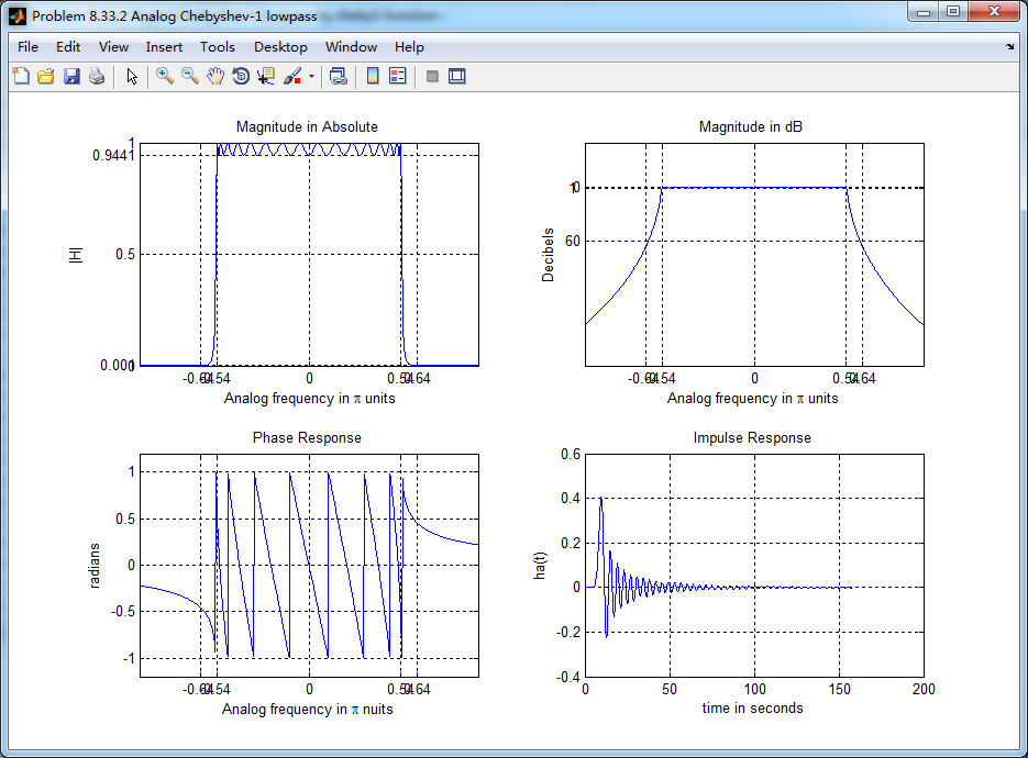
figure('NumberTitle', 'off', 'Name', 'Problem 8.33.2 Analog Chebyshev-1 lowpass')
set(gcf,'Color','white');
M = 1; % Omega max
subplot(2,2,1); plot(ww_s/pi, mag_s); grid on; %axis([-M, M, 0, 1.2]);
xlabel(' Analog frequency in pi units'); ylabel('|H|'); title('Magnitude in Absolute');
set(gca, 'XTickMode', 'manual', 'XTick', [-0.6366, -0.5437, 0, 0.5437, 0.6366]);
set(gca, 'YTickMode', 'manual', 'YTick', [0, 0.001, 0.5, 0.9441, 1]);
subplot(2,2,2); plot(ww_s/pi, db_s); grid on; %axis([0, M, -50, 10]);
xlabel('Analog frequency in pi units'); ylabel('Decibels'); title('Magnitude in dB ');
set(gca, 'XTickMode', 'manual', 'XTick', [-0.6366, -0.5437, 0, 0.5437, 0.6366]);
set(gca, 'YTickMode', 'manual', 'YTick', [-65, -60, -1, 0]);
set(gca,'YTickLabelMode','manual','YTickLabel',[ '65'; '60';'1 ';' 0']);
subplot(2,2,3); plot(ww_s/pi, pha_s/pi); grid on; axis([-M, M, -1.2, 1.2]);
xlabel('Analog frequency in pi nuits'); ylabel('radians'); title('Phase Response');
set(gca, 'XTickMode', 'manual', 'XTick', [-0.6366, -0.5437, 0, 0.5437, 0.6366]);
set(gca, 'YTickMode', 'manual', 'YTick', [-1:0.5:1]);
subplot(2,2,4); plot(t, ha); grid on; %axis([0, 30, -0.05, 0.25]);
xlabel('time in seconds'); ylabel('ha(t)'); title('Impulse Response');
figure('NumberTitle', 'off', 'Name', 'Problem 8.33.2 Digital Chebyshev-1 lowpass by afd_chb1 function')
set(gcf,'Color','white');
M = 2; % Omega max
subplot(2,2,1); plot(ww/pi, mag); axis([0, M, 0, 1.2]); grid on;
xlabel('Digital frequency in pi units'); ylabel('|H|'); title('Magnitude Response');
set(gca, 'XTickMode', 'manual', 'XTick', [0, 0.45, 0.50, 1.0, 1.5, 1.55, M]);
set(gca, 'YTickMode', 'manual', 'YTick', [0, 0.001, 0.5, 0.9441, 1]);
subplot(2,2,2); plot(ww/pi, pha/pi); axis([0, M, -1.1, 1.1]); grid on;
xlabel('Digital frequency in pi nuits'); ylabel('radians in pi units'); title('Phase Response');
set(gca, 'XTickMode', 'manual', 'XTick', [0, 0.45, 0.50, 1.0, M]);
set(gca, 'YTickMode', 'manual', 'YTick', [-1:1:1]);
subplot(2,2,3); plot(ww/pi, db); axis([0, M, -100, 10]); grid on;
xlabel('Digital frequency in pi units'); ylabel('Decibels'); title('Magnitude in dB ');
set(gca, 'XTickMode', 'manual', 'XTick', [0, 0.45, 0.50, 1.0, M]);
set(gca, 'YTickMode', 'manual', 'YTick', [-65, -60, -1, 0]);
set(gca,'YTickLabelMode','manual','YTickLabel',['65'; '60';' 1';' 0']);
subplot(2,2,4); plot(ww/pi, grd); grid on; axis([0, M, 0, 200]);
xlabel('Digital frequency in pi units'); ylabel('Samples'); title('Group Delay');
set(gca, 'XTickMode', 'manual', 'XTick', [0, 0.45, 0.50, 1.0, M]);
%set(gca, 'YTickMode', 'manual', 'YTick', [0:20:100]);
figure('NumberTitle', 'off', 'Name', 'Problem 8.33.2 Pole-Zero Plot')
set(gcf,'Color','white');
zplane(b,a);
title(sprintf('Pole-Zero Plot'));
%pzplotz(b,a);
% ---------------------------------------------------------------
% method 2: MATLAB cheby1 function
% ---------------------------------------------------------------
% Analog Prototype Order Calculations:
ep = sqrt(10^(Rp/10)-1); % Passband Ripple Factor
A = 10^(As/20); % Stopband Attenuation Factor
OmegaC = OmegaP; % Analog Chebyshev-1 prototype cutoff freq
OmegaR = OmegaS/OmegaP; % Analog prototype Transition ratio
g = sqrt(A*A-1)/ep; % Analog prototype Intermediate cal
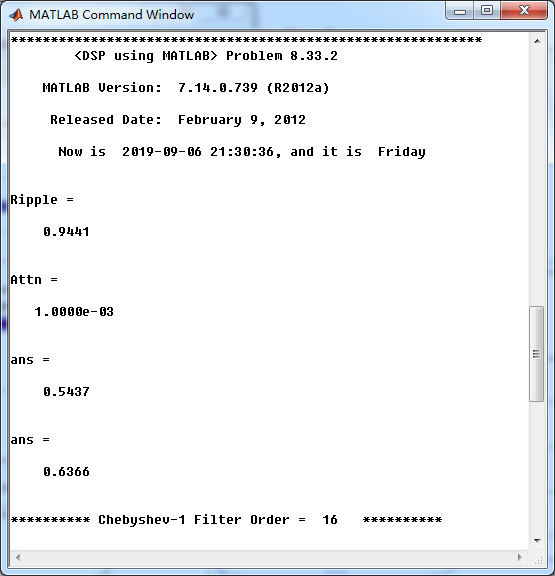
N = ceil(log10(g+sqrt(g*g-1))/log10(OmegaR+sqrt(OmegaR*OmegaR-1)));
fprintf('
********** Chebyshev-I Filter Order = %3.0f
', N)
% Digital Chebyshev-1 Filter Design:
wn = wp/pi; % Digital Chebyshev-1 cutoff freq in pi units
[b, a] = cheby1(N, Rp, wn); [C, B, A] = dir2cas(b, a)
% Calculation of Frequency Response:
[db, mag, pha, grd, ww] = freqz_m(b, a);
delta_w = 2*pi/1000;
Rp = -(min(db(1:1:ceil(wp/delta_w)+1))); % Actual Passband Ripple
fprintf('
Actual Passband Ripple is %.4f dB.
', Rp);
As = -round(max(db(ceil(ws/delta_w)+1:1:501))); % Min Stopband attenuation
fprintf('
Min Stopband attenuation is %.4f dB.
', As);
%% -----------------------------------------------------------------
%% Plot
%% -----------------------------------------------------------------
figure('NumberTitle', 'off', 'Name', 'Problem 8.33.2 Digital Chebyshev-1 lowpass by cheby1 function')
set(gcf,'Color','white');
M = 2; % Omega max
subplot(2,2,1); plot(ww/pi, mag); axis([0, M, 0, 1.2]); grid on;
xlabel('Digital frequency in pi units'); ylabel('|H|'); title('Magnitude Response');
set(gca, 'XTickMode', 'manual', 'XTick', [0, 0.45, 0.50, 1, M]);
set(gca, 'YTickMode', 'manual', 'YTick', [0, 0.001, 0.9441, 1]);
subplot(2,2,2); plot(ww/pi, pha/pi); axis([0, M, -1.1, 1.1]); grid on;
xlabel('Digital frequency in pi nuits'); ylabel('radians in pi units'); title('Phase Response');
set(gca, 'XTickMode', 'manual', 'XTick', [0, 0.45, 0.50, 1, M]);
set(gca, 'YTickMode', 'manual', 'YTick', [-1:1:1]);
subplot(2,2,3); plot(ww/pi, db); axis([0, M, -100, 10]); grid on;
xlabel('Digital frequency in pi units'); ylabel('Decibels'); title('Magnitude in dB ');
set(gca, 'XTickMode', 'manual', 'XTick', [0, 0.45, 0.50, 1, M]);
set(gca, 'YTickMode', 'manual', 'YTick', [-70, -60, -15, -1, 0]);
set(gca,'YTickLabelMode','manual','YTickLabel',['70'; '60';'15';' 1';' 0']);
subplot(2,2,4); plot(ww/pi, grd); axis([0, M, 0, 150]); grid on;
xlabel('Digital frequency in pi units'); ylabel('Samples'); title('Group Delay');
set(gca, 'XTickMode', 'manual', 'XTick', [0, 0.45, 0.50, 1, M]);
set(gca, 'YTickMode', 'manual', 'YTick', [0:20:100]);
% ----------------------------------------------
% Calculation of Impulse Response
% ----------------------------------------------
figure('NumberTitle', 'off', 'Name', 'Problem 8.33.2 Imp & Freq Response')
set(gcf,'Color','white');
t = [0:0.5:160]; subplot(2,1,1); impulse(cs,ds,t); grid on; % Impulse response of the analog filter
axis([0,160,-0.4,0.5]);hold on
n = [0:1:160/T]; hn = filter(b,a,impseq(0,0,160/T)); % Impulse response of the digital filter
stem(n*T,hn); xlabel('time in sec'); title (sprintf('Impulse Responses, T=%f',T));
hold off
% Calculation of Frequency Response:
[dbs, mags, phas, wws] = freqs_m(cs, ds, 2*pi/T); % Analog frequency s-domain
[dbz, magz, phaz, grdz, wwz] = freqz_m(b, a); % Digital z-domain
%% -----------------------------------------------------------------
%% Plot
%% -----------------------------------------------------------------
subplot(2,1,2); plot(wws/(2*pi), mags*Fs, 'b', wwz/(2*pi)*Fs, magz,'r'); grid on;
xlabel('frequency in Hz'); title('Magnitude Responses'); ylabel('Magnitude');
text(-0.3,0.15,'Analog filter', 'Color', 'b'); text(0.4,0.55,'Digital filter', 'Color', 'r');
运行结果:
这里只放chebyshev-1型,第2小题
通带、阻带绝对指标,以及模拟滤波器频带截止频率,
模拟chebyshev-1型低通滤波器,幅度谱、相位谱和脉冲响应
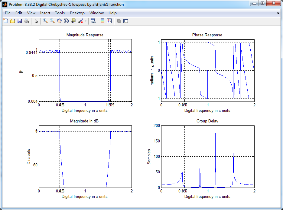
采用afd_chb1函数(双线性变换法),得到数字chebyshev-1低通滤波器,其幅度谱、相位谱和群延迟响应
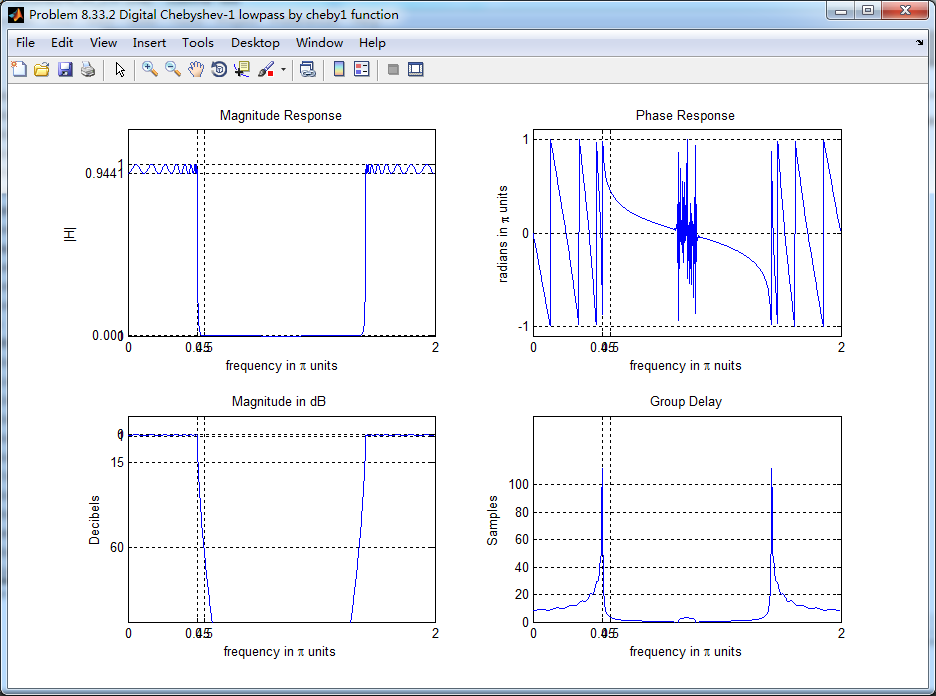
采用MATLAB自带cheby1函数,得到数字低通,幅度谱、相位谱和群延迟响应
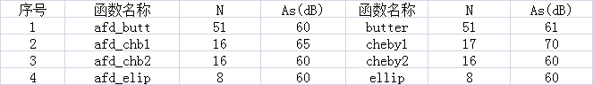
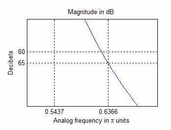
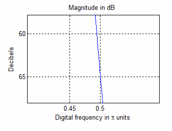
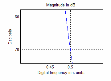
以下三图是模拟低通、两函数得到数字低通,各自最低阻带衰减对比,可见,MATLAB自带的cheby1函数设计的数字低通可以达到70dB。
至于其它的代码这里不放了,步骤类似,最后给出设计滤波器阶数和阻带衰减对比结果