bilibili莫烦tensorflow视频教程学习笔记
1.初次使用Tensorflow实现一元线性回归
# 屏蔽警告
import os
os.environ['TF_CPP_MIN_LOG_LEVEL'] = '2'

import numpy as np
import tensorflow as tf

# create dataset
x_data = np.random.rand(100).astype(np.float32)
y_data = x_data * 2 + 5

### create tensorflow structure Start
# 初始化Weights变量,由于是一元变量,所以w也只有一个
Weights = tf.Variable(tf.random_uniform([1],-1.0,1.0))
# 初始化bias,即截距b
biases = tf.Variable(tf.zeros([1]))

# 计算预测的y值,即y hat
y = Weights*x_data+biases

# 计算损失值
loss = tf.reduce_mean(tf.square(y-y_data))

# 优化器,这里采用普通的梯度下降,学习率alpha=0.5(0,1范围)
optimizer = tf.train.GradientDescentOptimizer(0.5)
# 使用优化器开始训练loss
train = optimizer.minimize(loss)

# tensorflow初始化变量
init = tf.global_variables_initializer()

# create tensorflow structure End

# 创建tensorflow的Session
sess = tf.Session()
# 激活initialize,很重要
sess.run(init)

# 运行两百轮
for step in range(201):
    # 执行一次训练
    sess.run(train)
    # 每20轮打印一次Wights和biases,看其变化
    if step % 20 ==0:
        print(step,sess.run(Weights),sess.run(biases))
os.environ['TF_CPP_MIN_LOG_LEVEL'] = '2' 解释:
TF_CPP_MIN_LOG_LEVEL = 0:0为默认值,输出所有的信息,包含info,warning,error,fatal四种级别
TF_CPP_MIN_LOG_LEVEL = 1:1表示屏蔽info,只显示warning及以上级别
TF_CPP_MIN_LOG_LEVEL = 2:2表示屏蔽info和warning,显示error和fatal(最常用的取值)
TF_CPP_MIN_LOG_LEVEL = 3:3表示只显示fatal
2.Tensorflow基础 基本流程
# 导入tensorflow,安装的GPU版本,则默认使用GPU
import tensorflow as tf

# 定义两个矩阵常量
matrix1 = tf.constant([[3, 3], [2, 4]])
matrix2 = tf.constant([[1, 2], [5, 5]])
# 矩阵乘法,相当于np.dot(mat1,mat2)
product = tf.matmul(matrix1, matrix2)
# 初始化
init = tf.global_variables_initializer()
# 使用with来定义Session,这样使用完毕后会自动sess.close()
with tf.Session() as sess:
    # 执行初始化
    sess.run(init)
    # 打印结果
    result = sess.run(product)
    print(result)
3.tensorflow基础 变量、常量、传值
import tensorflow as tf

state = tf.Variable(0, name='counter')
one = tf.constant(1)

# 变量state和常量one相加
new_value = tf.add(state, one)
# 将new_value赋值给state
update = tf.assign(state, new_value)
# 初始化全局变量
init = tf.global_variables_initializer()
# 打开Session
with tf.Session() as sess:
    # 执行初始化,很重要
    sess.run(init)
    # 运行三次update
    for _ in range(3):
        sess.run(update)
        print(sess.run(state))
4.使用placeholder
import tensorflow as tf

# 使用placeholder定义两个空间,用于存放float32的数据
input1 = tf.placeholder(tf.float32)
input2 = tf.placeholder(tf.float32)
# 计算input1和input2的乘积
output = tf.matmul(input1, input2)

# 定义sess
with tf.Session() as sess:
    # 运行output,并在run的时候喂入数据
    print(sess.run(output, feed_dict={input1: [[2.0, 3.0]], input2: [[4.0], [2.0]]}))
5.定义一个层(Layer)
import tensorflow as tf

# inputs是上一层的输出,insize是上一层的节点数,outsize是本层节点数,af是激活函数,默认
# 为线性激活函数,即f(x)=X
def add_layer(inputs, in_size, out_size, activation_function=None):
    # 定义权重w,并且用随机值填充,大小为in_size*out_size
    Weights = tf.Variable(tf.random_normal([in_size, out_size]))
    # 定义变差bias,大小为1*out_size
    biases = tf.Variable(tf.zeros([1, out_size]) + 0.1)
    # 算出z=wx+b
    Wx_plus_b = tf.matmul(inputs, Weights) + biases
    # 如果激励函数为空,则使用线性激励函数
    if activation_function is None:
        outputs = Wx_plus_b
    else:
        # 如果不为空,则使用激励方程activation_function()
        outputs = activation_function(Wx_plus_b)
    # 返回输出值
    return outputs
6.手动创建一个简单的神经网络
(包含一个输入层、一个隐藏层、一个输出层)
import numpy as np
import tensorflow as tf


# 添加一个隐藏层
def add_layer(inputs, in_size, out_size, activation_function=None):
    Weights = tf.Variable(tf.random_normal([in_size, out_size]))
    biases = tf.Variable(tf.zeros([1, out_size]) + 0.1)
    Wx_plus_b = tf.matmul(inputs, Weights) + biases
    if activation_function is None:
        outputs = Wx_plus_b
    else:
        outputs = activation_function(Wx_plus_b)
    return outputs


### 准备数据
# 创建x_data,从-1到1,分成300份,然后添加维度,让其编程一个300*1的矩阵
x_data = np.linspace(-1, 1, 300)[:, np.newaxis]
# 定义一个噪声矩阵,大小和x_data一样,数据均值为0,方差为0.05
noise = np.random.normal(0, 0.05, x_data.shape)
# 按公式x^2-0.5计算y_data,并加上噪声
y_data = np.square(x_data) - 0.5 + noise

# 定义两个placeholder分别用于传入x_data和y_data
xs = tf.placeholder(tf.float32, [None, 1])
ys = tf.placeholder(tf.float32, [None, 1])

# 创建一个隐藏层,输入为xs,输入层只有一个节点,本层有10个节点,激励函数为relu
l1 = add_layer(xs, 1, 10, activation_function=tf.nn.relu)
# 创建输出层
prediction = add_layer(l1, 10, 1, activation_function=None)

# 定义损失
loss = tf.reduce_mean(tf.reduce_sum(tf.square(ys - prediction),
                                    reduction_indices=[1]))
# 使用梯度下降对loss进行最小化,学习率为0.01
train_step = tf.train.GradientDescentOptimizer(0.01).minimize(loss)
# 初始化全局变量
init = tf.global_variables_initializer()
# 创建Session
with tf.Session() as sess:
    # 初始化
    sess.run(init)
    # 运行10000轮梯度下降
    for _ in range(10001):
        sess.run(train_step, feed_dict={xs: x_data, ys: y_data})
        # 每50轮打印一下loss看是否在减小
        if _ % 50 == 0:
            print(sess.run(loss, feed_dict={xs: x_data, ys: y_data}))
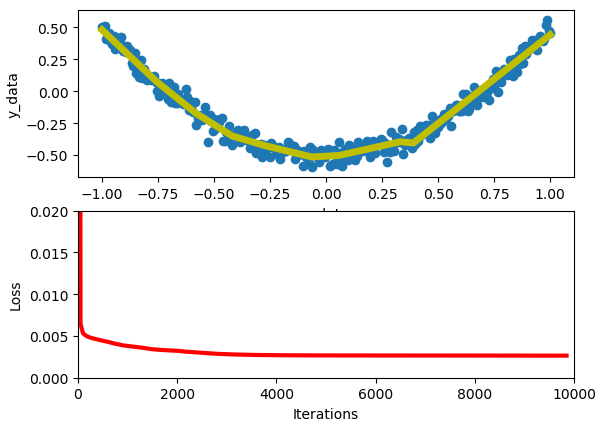
7.使用matplotlib可视化拟合情况、Loss曲线
import numpy as np
import tensorflow as tf
import matplotlib.pyplot as plt


# 添加一个隐藏层
def add_layer(inputs, in_size, out_size, activation_function=None):
    Weights = tf.Variable(tf.random_normal([in_size, out_size]))
    biases = tf.Variable(tf.zeros([1, out_size]) + 0.1)
    Wx_plus_b = tf.matmul(inputs, Weights) + biases
    if activation_function is None:
        outputs = Wx_plus_b
    else:
        outputs = activation_function(Wx_plus_b)
    return outputs


### 准备数据
# 创建x_data,从-1到1,分成300份,然后添加维度,让其编程一个300*1的矩阵
x_data = np.linspace(-1, 1, 300)[:, np.newaxis]
# 定义一个噪声矩阵,大小和x_data一样,数据均值为0,方差为0.05
noise = np.random.normal(0, 0.05, x_data.shape)
# 按公式x^2-0.5计算y_data,并加上噪声
y_data = np.square(x_data) - 0.5 + noise

# 定义两个placeholder分别用于传入x_data和y_data
xs = tf.placeholder(tf.float32, [None, 1])
ys = tf.placeholder(tf.float32, [None, 1])

# 创建一个隐藏层,输入为xs,输入层只有一个节点,本层有10个节点,激励函数为relu
l1 = add_layer(xs, 1, 10, activation_function=tf.nn.relu)
# 创建输出层
prediction = add_layer(l1, 10, 1, activation_function=None)

# 定义损失
loss = tf.reduce_mean(tf.reduce_sum(tf.square(ys - prediction),
                                    reduction_indices=[1]))
# 使用梯度下降对loss进行最小化,学习率为0.01
train_step = tf.train.GradientDescentOptimizer(0.1).minimize(loss)
# 初始化全局变量
init = tf.global_variables_initializer()
# 创建Session
with tf.Session() as sess:
    # 初始化
    sess.run(init)

    # 创建图形
    fig = plt.figure()
    # 创建子图,上下两个图的第一个(行,列,子图编号),用于画拟合图
    a1 = fig.add_subplot(2, 1, 1)
    # 使用x_data,y_data画散点图
    plt.scatter(x_data, y_data)
    plt.xlabel('x_data')
    plt.ylabel('y_data')
    # 修改图形x,y轴上下限x limit,y limit
    # plt.xlim(-2, 2)
    # plt.ylim(-1, 1)
    # 也可以用一行代码修改plt.axis([-2,2,-1,1])
    plt.axis('tight')  # 可以按内容自动收缩,不留空白

    # 创建第二个子图,用于画Loss曲线
    a2 = fig.add_subplot(2, 1, 2)
    # 可以使用这种方式来一次性设置子图的属性,和使用plt差不多
    a2.set(xlim=(0, 10000), ylim=(0.0, 0.02), xlabel='Iterations', ylabel='Loss')

    # 使用plt.ion使其运行show()后不暂停
    plt.ion()
    # 展示图片,必须使用show()
    plt.show()

    loss_list = []
    index_list = []

    # 运行10000轮梯度下降
    for _ in range(10001):
        sess.run(train_step, feed_dict={xs: x_data, ys: y_data})
        # 每50轮打印一下loss看是否在减小
        if _ % 50 == 0:
            index_list.append(_)
            loss_list.append(sess.run(loss, feed_dict={xs: x_data, ys: y_data}))

            # 避免在图中重复的画线,线尝试删除已经存在的线
            try:
                a1.lines.remove(lines_in_a1[0])
                a2.lines.remove(lines_in_a2[0])
            except Exception:
                pass

            prediction_value = sess.run(prediction, feed_dict={xs: x_data})
            # 在a1子图中画拟合线,黄色,宽度5
            lines_in_a1 = a1.plot(x_data, prediction_value, 'y-', lw=5)
            # 在a2子图中画Loss曲线,红色,宽度3
            lines_in_a2 = a2.plot(index_list, loss_list, 'r-', lw=3)
            # 暂停一下,否则会卡
            plt.pause(0.1)
注意:如果在pycharm运行上述代码,不能展示动态图片刷新,则需要进入File->setting,搜索Python Scientific,然后右侧去掉对勾(默认是勾选的),然后Apply,OK即可。
8.常用优化器Optimizers
train_step = tf.train.GradientDescentOptimizer(0.1).minimize(loss)
train_step = tf.train.AdamOptimizer(learning_rate=0.01, beta1=0.9, beta2=0.999, epsilon=1e-8).minimize(loss)
train_step = tf.train.MomentumOptimizer(learning_rate=0.01,momentum=0.9).minimize(loss)
train_step = tf.train.RMSPropOptimizer(learning_rate=0.01).minimize(loss)
其中Adam效果比较好,但都可以尝试使用。
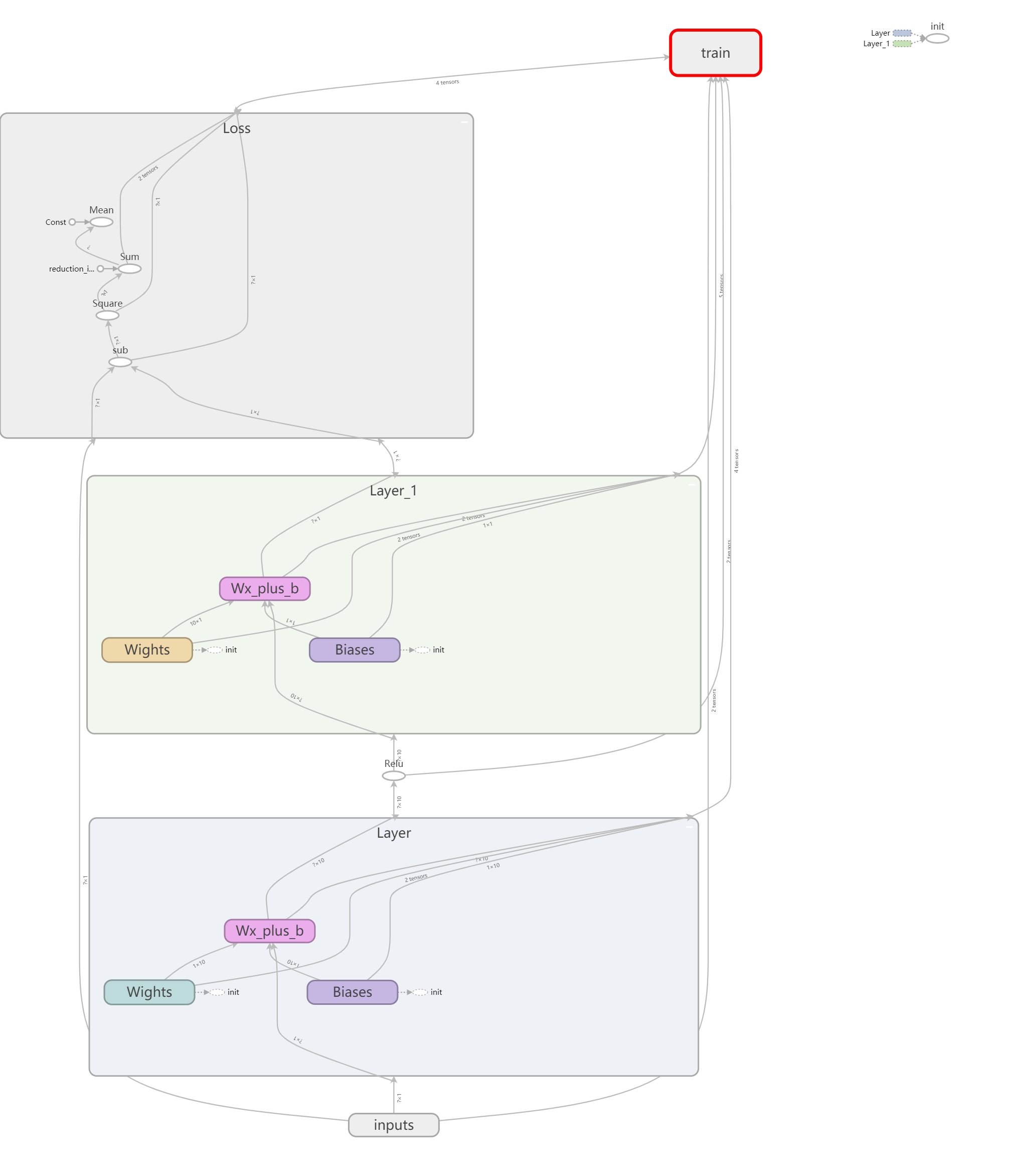
9.使用tensorboard绘网络结构图
import numpy as np
import tensorflow as tf


def add_layer(inputs, in_size, out_size, activation_function=None):
    # 每使用该函数创建一层,则生成一个名为Layer_n的外层框
    with tf.name_scope('Layer'):
        # 内层权重框
        with tf.name_scope('Wights'):
            Weights = tf.Variable(tf.random_normal([in_size, out_size]))
        # 内层Bias框
        with tf.name_scope('Biases'):
            biases = tf.Variable(tf.zeros([1, out_size]) + 0.1)
        # 内层z(x,w,b)框
        with tf.name_scope('Wx_plus_b'):
            Wx_plus_b = tf.matmul(inputs, Weights) + biases
    if activation_function is None:
        outputs = Wx_plus_b
    else:
        outputs = activation_function(Wx_plus_b)
    return outputs


# 准备数据
x_data = np.linspace(-1, 1, 300)[:, np.newaxis]
noise = np.random.normal(0, 0.05, x_data.shape)
y_data = np.square(x_data) - 0.5 + noise

# 使用tensorboard画inputs层
with tf.name_scope('inputs'):  # 一个名为inputs的外层框
    # x_input和y_input
    xs = tf.placeholder(tf.float32, [None, 1], name='x_input')
    ys = tf.placeholder(tf.float32, [None, 1], name='y_input')

l1 = add_layer(xs, 1, 10, activation_function=tf.nn.relu)
prediction = add_layer(l1, 10, 1, activation_function=None)

# Loss框,其中包含计算Loss的各个步骤,例如sub,square,sum,mean等
with tf.name_scope("Loss"):
    loss = tf.reduce_mean(tf.reduce_sum(tf.square(ys - prediction),
                                        reduction_indices=[1]))
# train框,其中包含梯度下降步骤和权重更新步骤
with tf.name_scope('train'):
    train_step = tf.train.GradientDescentOptimizer(0.1).minimize(loss)

init = tf.global_variables_initializer()

with tf.Session() as sess:
    # 将图写入文件夹logs
    writer = tf.summary.FileWriter('logs/')
    # 写入文件,名为events.out.tfevents.1561191707.06P2GHW85CAH236
    writer.add_graph(sess.graph)
    sess.run(init)
注意:在运行代码后,在logs文件夹下生成 events.out.tfevents.1561191707.06P2GHW85CAH236 文件。
然后进入windows cmd,进入logs的上层文件夹,使用tensorboard --logdir logs即可打开web服务,然后复制给出的url地址进行访问。如图:

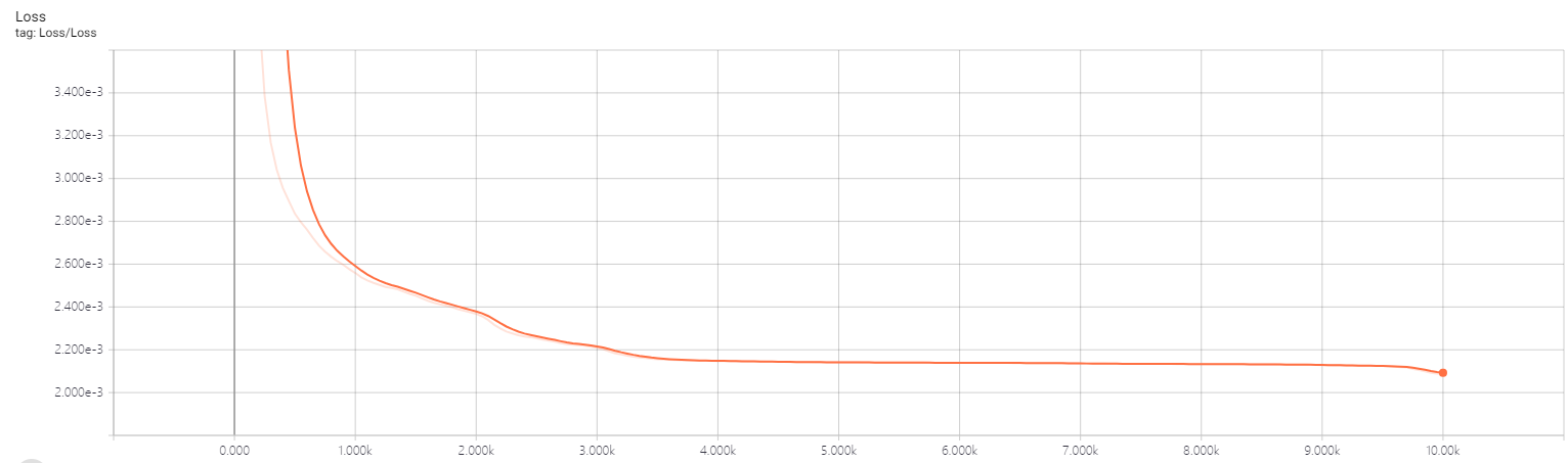
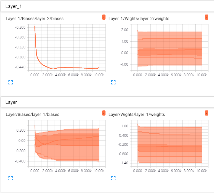
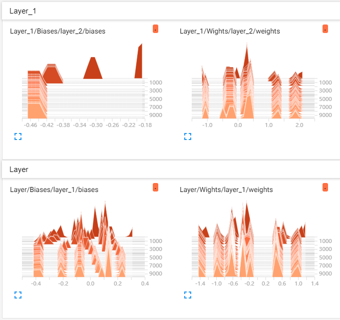
10.其他可视化,例如Weight、bias、loss等
import numpy as np
import tensorflow as tf


def add_layer(inputs, in_size, out_size, n_layer, activation_function=None):
    layer_name = 'layer_%d' % n_layer
    # 每使用该函数创建一层,则生成一个名为Layer_n的外层框
    with tf.name_scope('Layer'):

        # 内层权重框
        with tf.name_scope('Wights'):
            Weights = tf.Variable(tf.random_normal([in_size, out_size]), name='W')
            tf.summary.histogram(layer_name + '/weights', Weights)
        # 内层Bias框
        with tf.name_scope('Biases'):
            biases = tf.Variable(tf.zeros([1, out_size]) + 0.1, name='B')
            tf.summary.histogram(layer_name + '/biases', biases)
        # 内层z(x,w,b)框
        with tf.name_scope('Wx_plus_b'):
            Wx_plus_b = tf.matmul(inputs, Weights) + biases
    if activation_function is None:
        outputs = Wx_plus_b
    else:
        outputs = activation_function(Wx_plus_b)
    return outputs


# 准备数据
x_data = np.linspace(-1, 1, 300)[:, np.newaxis]
noise = np.random.normal(0, 0.05, x_data.shape)
y_data = np.square(x_data) - 0.5 + noise

# 使用tensorboard画inputs层
with tf.name_scope('inputs'):  # 一个名为inputs的外层框
    # x_input和y_input
    xs = tf.placeholder(tf.float32, [None, 1], name='x_input')
    ys = tf.placeholder(tf.float32, [None, 1], name='y_input')

l1 = add_layer(xs, 1, 10, 1, activation_function=tf.nn.relu)
prediction = add_layer(l1, 10, 1, 2, activation_function=None)

# Loss框,其中包含计算Loss的各个步骤,例如sub,square,sum,mean等
with tf.name_scope("Loss"):
    loss = tf.reduce_mean(tf.reduce_sum(tf.square(ys - prediction),
                                        reduction_indices=[1]))
    tf.summary.scalar('Loss', loss)
# train框,其中包含梯度下降步骤和权重更新步骤
with tf.name_scope('train'):
    train_step = tf.train.GradientDescentOptimizer(0.1).minimize(loss)

init = tf.global_variables_initializer()

merged = tf.summary.merge_all()

with tf.Session() as sess:
    # 将图写入文件夹logs
    writer = tf.summary.FileWriter('logs/')
    # 写入文件,名为events.out.tfevents.1561191707.06P2GHW85CAH236
    writer.add_graph(sess.graph)
    sess.run(init)

    # 运行10000轮梯度下降
    for _ in range(10001):
        sess.run(train_step, feed_dict={xs: x_data, ys: y_data})
        # 每50步在loss曲线中记一个点
        if _ % 50 == 0:
            # 将merged和步数加入到总结中
            result = sess.run(merged, feed_dict={xs: x_data, ys: y_data})
            writer.add_summary(result, _)
11.使用tensorflow进行Mnist分类
import tensorflow as tf
from tensorflow.examples.tutorials.mnist import input_data

mnist = input_data.read_data_sets('MNIST_data', one_hot=True)


# 添加一个隐藏层
def add_layer(inputs, in_size, out_size, activation_function=None):
    Weights = tf.Variable(tf.random_normal([in_size, out_size]))
    biases = tf.Variable(tf.zeros([1, out_size]) + 0.1)
    Wx_plus_b = tf.matmul(inputs, Weights) + biases
    if activation_function is None:
        outputs = Wx_plus_b
    else:
        outputs = activation_function(Wx_plus_b)
    return outputs


# 测试准确度accuracy
def compute_accuracy(v_xs, v_ys):
    # 引入全局变量prediction层
    global prediction
    # 用v_xs输入数据跑一次prediction层,得到输出
    y_pre = sess.run(prediction, feed_dict={xs: v_xs})
    # 对比输出和数据集label,相同的为1,不同的为0
    correct_prediction = tf.equal(tf.argmax(y_pre, 1), tf.argmax(v_ys, 1))
    # 计算比对结果,可得到准确率百分比
    accuracy = tf.reduce_mean(tf.cast(correct_prediction, tf.float32))
    # 获取result,并返回
    result = sess.run(accuracy, feed_dict={xs: v_xs, ys: v_ys})
    return result


# define placeholder for inputs on network
xs = tf.placeholder(tf.float32, [None, 784])  # 手写数字的图片大小为28*28
ys = tf.placeholder(tf.float32, [None, 10])  # 输出为1*10的Onehot热独

# 只有一个输出层,输入为m*784的数据,输出为m*10的数据,m=100,因为batch_size取的是100
prediction = add_layer(xs, 784, 10, activation_function=tf.nn.softmax)

# 使用交叉熵损失函数g(x)=-E[y*log(y_hat)],y为ys,例如[0,1,0,0,0,0,0,0,0,0],即数字为1,
# 假设y_hat=[0.05,0.81,0.05,0.003,0.012,0.043,0.012,0.009,0.006,0.005],
# 则g(x) = -(0*log0.05+1*log0.81+...+0*log0.005)=-log0.81=0.0915
# g(x)就是-tf.reduce_sum(ys * tf.log(prediction)
# tf.reduce_mean(g(x),reduction_indices=[1])是对一个batch_size的样本取平均损失
# 相当于1/m * E(1 to m) [g(x)]
cross_entropy = tf.reduce_mean(-tf.reduce_sum(ys * tf.log(prediction),
                                              reduction_indices=[1]))
# 使用梯度下降,学习率为0.5来最小化cross_entropy
train_step = tf.train.GradientDescentOptimizer(0.5).minimize(cross_entropy)

# 定义Session
sess = tf.Session()
# 初始化
sess.run(tf.global_variables_initializer())
# 跑10000轮
for i in range(10001):
    # 使用SGD,batch_size=100
    batch_x, batch_y = mnist.train.next_batch(100)
    # 执行一轮
    sess.run(train_step, feed_dict={xs: batch_x, ys: batch_y})
    # 每跑50轮打印一次准确度
    if i % 50 == 0:
        # 训练集准确度
        print('TRAIN acc:', compute_accuracy(
            batch_x, batch_y))
        # 测试集准确度
        print('TEST acc:', compute_accuracy(
            mnist.test.images, mnist.test.labels))
重点:关注代码中交叉熵损失函数的使用,多分类时的交叉熵损失函数为L(y_hat,y)=-E(j=1 to k) yj*log y_hatj,成本函数为J = 1/m E(i=1 to m) L(y_hati,yi)
12.使用Dropout避免过拟合
import tensorflow as tf
from tensorflow.examples.tutorials.mnist import input_data

mnist = input_data.read_data_sets('MNIST_data', one_hot=True)


# 添加一个隐藏层
def add_layer(inputs, in_size, out_size, activation_function=None, keep_prob=1):
    Weights = tf.Variable(tf.random_normal([in_size, out_size]))
    biases = tf.Variable(tf.zeros([1, out_size]) + 0.1)
    Wx_plus_b = tf.matmul(inputs, Weights) + biases
    # 这里使用Dropout处理计算结果,默认keep_prob为1,具体drop比例按1-keep_prob执行
    Wx_plus_b = tf.nn.dropout(Wx_plus_b, keep_prob)

    if activation_function is None:
        outputs = Wx_plus_b
    else:
        outputs = activation_function(Wx_plus_b)
    return outputs


# 测试准确度accuracy
def compute_accuracy(v_xs, v_ys):
    # 引入全局变量prediction层
    global prediction
    # 用v_xs输入数据跑一次prediction层,得到输出
    y_pre = sess.run(prediction, feed_dict={xs: v_xs})
    # 对比输出和数据集label,相同的为1,不同的为0
    correct_prediction = tf.equal(tf.argmax(y_pre, 1), tf.argmax(v_ys, 1))
    # 计算比对结果,可得到准确率百分比
    accuracy = tf.reduce_mean(tf.cast(correct_prediction, tf.float32))
    # 获取result,并返回
    result = sess.run(accuracy, feed_dict={xs: v_xs, ys: v_ys})
    return result


# define placeholder for inputs on network
xs = tf.placeholder(tf.float32, [None, 784])  # 手写数字的图片大小为28*28
ys = tf.placeholder(tf.float32, [None, 10])  # 输出为1*10的Onehot热独

# 创建一个隐层,有50个节点,使用Dropout 30%来避免过拟合
l1 = add_layer(xs, 784, 50, activation_function=tf.nn.tanh, keep_prob=0.7)
# 创建输出层,输入为m*784的数据,输出为m*10的数据,m=100,因为batch_size取的是100
prediction = add_layer(l1, 50, 10, activation_function=tf.nn.softmax)

# 使用交叉熵损失函数g(x)=-E[y*log(y_hat)],y为ys,例如[0,1,0,0,0,0,0,0,0,0],即数字为1,
# 假设y_hat=[0.05,0.81,0.05,0.003,0.012,0.043,0.012,0.009,0.006,0.005],
# 则g(x) = -(0*log0.05+1*log0.81+...+0*log0.005)=-log0.81=0.0915
# g(x)就是-tf.reduce_sum(ys * tf.log(prediction)
# tf.reduce_mean(g(x),reduction_indices=[1])是对一个batch_size的样本取平均损失
# 相当于1/m * E(1 to m) [g(x)]
cross_entropy = tf.reduce_mean(-tf.reduce_sum(ys * tf.log(prediction),
                                              reduction_indices=[1]))
tf.summary.scalar('Loss', cross_entropy)

# 使用梯度下降,学习率为0.5来最小化cross_entropy
train_step = tf.train.GradientDescentOptimizer(0.5).minimize(cross_entropy)

# 定义Session
sess = tf.Session()

# 创建连个graph,图是重合的,即可以再loss曲线中同时画出train和test数据集的loss曲线,从而看是否存在过拟合
train_writer = tf.summary.FileWriter('logs/train', sess.graph)
test_writer = tf.summary.FileWriter('logs/test', sess.graph)

merged = tf.summary.merge_all()

# 初始化
sess.run(tf.global_variables_initializer())
# 跑10000轮
for i in range(20001):
    # 使用SGD,batch_size=100
    batch_x, batch_y = mnist.train.next_batch(100)
    # 执行一轮
    sess.run(train_step, feed_dict={xs: batch_x, ys: batch_y})
    # 每跑50轮打印一次准确度
    if i % 50 == 0:
        train_res = sess.run(merged, feed_dict={xs: mnist.train.images, ys: mnist.train.labels})
        test_res = sess.run(merged, feed_dict={xs: mnist.test.images, ys: mnist.test.labels})
        train_writer.add_summary(train_res, i)
        test_writer.add_summary(test_res, i)
重点:在创建每个层时,如果需要Dropout,就给他一个keep_prob,然后使用tf.nn.dropout(result,keep_prob)来执行Dropout。
13.tensorflow中使用卷积网络分类Mnist
import os

import tensorflow as tf
from tensorflow.examples.tutorials.mnist import input_data

os.environ['TF_CPP_MIN_LOG_LEVEL'] = '2'
mnist = input_data.read_data_sets('MNIST_data', one_hot=True)


# 添加一个隐藏层
def add_layer(inputs, in_size, out_size, activation_function=None, keep_prob=1):
    Weights = tf.Variable(tf.random_normal([in_size, out_size]))
    biases = tf.Variable(tf.zeros([1, out_size]) + 0.1)
    Wx_plus_b = tf.matmul(inputs, Weights) + biases
    # 这里使用Dropout处理计算结果,默认keep_prob为1,具体drop比例按1-keep_prob执行
    Wx_plus_b = tf.nn.dropout(Wx_plus_b, keep_prob)

    if activation_function is None:
        outputs = Wx_plus_b
    else:
        outputs = activation_function(Wx_plus_b)
    return outputs


# 测试准确度accuracy
def compute_accuracy(v_xs, v_ys):
    # 引入全局变量prediction层
    global prediction
    # 用v_xs输入数据跑一次prediction层,得到输出
    y_pre = sess.run(prediction, feed_dict={xs: v_xs})
    # argmax(y,1)按行获取最大值的index
    # 对比输出和数据集label,相同的为1,不同的为0
    correct_prediction = tf.equal(tf.argmax(y_pre, 1), tf.argmax(v_ys, 1))
    # 计算比对结果,可得到准确率百分比
    accuracy = tf.reduce_mean(tf.cast(correct_prediction, tf.float32))
    # 获取result,并返回
    result = sess.run(accuracy, feed_dict={xs: v_xs, ys: v_ys})
    return result


# 按shape参数创建参数W矩阵
def weight_variable(shape):
    initial = tf.truncated_normal(shape, stddev=0.1)
    return tf.Variable(initial)


# 按shape参数创建bias矩阵
def bias_variable(shape):
    initial = tf.constant(0.1, shape=shape)
    return tf.Variable(initial)


# 创建2d卷积层,直接调用tf.nn.conv2d,x为输入,W为参数矩阵,strides=[1,y_step,x_step,1]
# padding有两个取值'SAME'和'VALID',对应一个填充,一个不填充
def conv2d(x, W):
    return tf.nn.conv2d(x, W, strides=[1, 1, 1, 1], padding='SAME')


# 创建最大池化层,ksize=[1,y_size,x_size,1],strides同上,padding同上
def max_pool_2x2(x):
    return tf.nn.max_pool(x, ksize=[1, 2, 2, 1], strides=[1, 2, 2, 1], padding='SAME')


# define placeholder for inputs on network
xs = tf.placeholder(tf.float32, [None, 784])  # 手写数字的图片大小为28*28
ys = tf.placeholder(tf.float32, [None, 10])  # 输出为1*10的Onehot热独
# 将数据的维度变化为图片的形式,[-1,28,28,1],-1表示样本数m(根据每轮训练的输入大小batch_size=100),28*28表示图片大小,1表示channel
x_data = tf.reshape(xs, [-1, 28, 28, 1])

###### 下面定义网络结构,大致根据Lenet的结构修改 ######
### 定义conv1层
# 定义conv layer1的Weights,[5,5,1,6]中得5*5表示核的大小,1表示核的channel,16表示核的个数
# 该矩阵为5*5*1*16的矩阵
W_conv1 = weight_variable([5, 5, 1, 16])
# 定义conv1的bias矩阵
b_conv1 = bias_variable([16])
# 定义conv1的激活函数
h_conv1 = tf.nn.relu(conv2d(x_data, W_conv1) + b_conv1)
# 定义池化层
h_pool1 = max_pool_2x2(h_conv1)

### 定义conv2层,参数参照conv1
W_conv2 = weight_variable([5, 5, 16, 32])
b_conv2 = bias_variable([32])
h_conv2 = tf.nn.relu(conv2d(h_pool1, W_conv2) + b_conv2)
h_pool2 = max_pool_2x2(h_conv2)
# 池化后要输入给后面的全连接层,所以要把7*7*32的矩阵压扁成[1568]的向量
h_pool2_flat = tf.reshape(h_pool2, [-1, 7 * 7 * 32])
# 检查一下矩阵维度,确认为(100,1568),其中100是batch_size
# h_shape = tf.shape(h_pool2_flat)

### 定义fc1层节点为200
# 定义fc1的weight矩阵,维度为1568*200
W_fc1 = weight_variable([7 * 7 * 32, 200])
# 200个bias
b_fc1 = bias_variable([200])
# fc层激活函数
h_fc1 = tf.nn.relu(tf.matmul(h_pool2_flat, W_fc1) + b_fc1)
# 是否启用dropout
# h_fc1_drop = tf.nn.dropout(h_fc1)

### 定义fc2层,参数参照fc1
W_fc2 = weight_variable([200, 100])
b_fc2 = bias_variable([100])
h_fc2 = tf.nn.relu(tf.matmul(h_fc1, W_fc2) + b_fc2)

### 定义输出层,激励函数不同
w_fc3 = weight_variable([100, 10])
b_fc3 = bias_variable([10])
# 输出层使用多分类softmax激励函数
prediction = tf.nn.softmax(tf.matmul(h_fc2, w_fc3) + b_fc3)

# 交叉熵损失
cross_entropy = tf.reduce_mean(-tf.reduce_sum(ys * tf.log(prediction),
                                              reduction_indices=[1]))
tf.summary.scalar('Loss', cross_entropy)

# 使用Adam优化算法,学习率为0.0001来最小化cross_entropy
train_step = tf.train.AdamOptimizer(1e-4).minimize(cross_entropy)

# 定义Session
sess = tf.Session()

# 创建连个graph,图是重合的,即可以再loss曲线中同时画出train和test数据集的loss曲线,从而看是否存在过拟合
train_writer = tf.summary.FileWriter('logs2/train', sess.graph)
test_writer = tf.summary.FileWriter('logs2/test', sess.graph)

merged = tf.summary.merge_all()

# 初始化
sess.run(tf.global_variables_initializer())
# 跑10000轮
for i in range(20001):
    # 使用SGD,batch_size=100
    batch_x, batch_y = mnist.train.next_batch(100)
    # 执行一轮
    sess.run(train_step, feed_dict={xs: batch_x, ys: batch_y})
    # 每跑50轮打印一次准确度
    if i % 100 == 0:
        train_res = sess.run(merged, feed_dict={xs: batch_x, ys: batch_y})
        test_res = sess.run(merged, feed_dict={xs: mnist.test.images, ys: mnist.test.labels})
        train_writer.add_summary(train_res, i)
        test_writer.add_summary(test_res, i)

        print('Acc on loop ', i, ':', compute_accuracy(mnist.test.images, mnist.test.labels))
在tensorflow 1.14.0下的代码如下(API更改较多):
# -*- coding:utf-8 -*-
__author__ = 'Leo.Z'

import tensorflow as tf
from tensorflow.examples.tutorials.mnist import input_data

import os

os.environ['TF_CPP_MIN_LOG_LEVEL'] = '2'

mnist = input_data.read_data_sets('MNIST_data', one_hot=True)


# 添加一个隐藏层
def add_layer(inputs, in_size, out_size, activation_function=None, keep_prob=1):
    Weights = tf.Variable(tf.random_normal([in_size, out_size]))
    biases = tf.Variable(tf.zeros([1, out_size]) + 0.1)
    Wx_plus_b = tf.matmul(inputs, Weights) + biases
    # 这里使用Dropout处理计算结果,默认keep_prob为1,具体drop比例按1-keep_prob执行
    Wx_plus_b = tf.nn.dropout(Wx_plus_b, keep_prob)

    if activation_function is None:
        outputs = Wx_plus_b
    else:
        outputs = activation_function(Wx_plus_b)
    return outputs


# 测试准确度accuracy
def compute_accuracy(v_xs, v_ys):
    # 引入全局变量prediction层
    global prediction
    # 用v_xs输入数据跑一次prediction层,得到输出
    y_pre = sess.run(prediction, feed_dict={xs: v_xs})
    # argmax(y,1)按行获取最大值的index
    # 对比输出和数据集label,相同的为1,不同的为0
    correct_prediction = tf.equal(tf.argmax(y_pre, 1), tf.argmax(v_ys, 1))
    # 计算比对结果,可得到准确率百分比
    accuracy = tf.reduce_mean(tf.cast(correct_prediction, tf.float32))
    # 获取result,并返回
    result = sess.run(accuracy, feed_dict={xs: v_xs, ys: v_ys})
    return result


# 按shape参数创建参数W矩阵
def weight_variable(shape):
    initial = tf.random.truncated_normal(shape, stddev=0.1)
    return tf.Variable(initial)


# 按shape参数创建bias矩阵
def bias_variable(shape):
    initial = tf.constant(0.1, shape=shape)
    return tf.Variable(initial)


# 创建2d卷积层,直接调用tf.nn.conv2d,x为输入,W为参数矩阵,strides=[1,y_step,x_step,1]
# padding有两个取值'SAME'和'VALID',对应一个填充,一个不填充
def conv2d(x, W):
    return tf.nn.conv2d(x, W, strides=[1, 1, 1, 1], padding='SAME')


# 创建最大池化层,ksize=[1,y_size,x_size,1],strides同上,padding同上
def max_pool_2x2(x):
    return tf.nn.max_pool2d(x, ksize=[1, 2, 2, 1], strides=[1, 2, 2, 1], padding='SAME')


# define placeholder for inputs on network
xs = tf.compat.v1.placeholder(tf.float32, [None, 784])  # 手写数字的图片大小为28*28
ys = tf.compat.v1.placeholder(tf.float32, [None, 10])  # 输出为1*10的Onehot热独
# 将数据的维度变化为图片的形式,[-1,28,28,1],-1表示样本数m(根据每轮训练的输入大小batch_size=100),28*28表示图片大小,1表示channel
x_data = tf.reshape(xs, [-1, 28, 28, 1])

###### 下面定义网络结构,大致根据Lenet的结构修改 ######
### 定义conv1层
# 定义conv layer1的Weights,[5,5,1,6]中得5*5表示核的大小,1表示核的channel,16表示核的个数
# 该矩阵为5*5*1*16的矩阵
W_conv1 = weight_variable([5, 5, 1, 16])
# 定义conv1的bias矩阵
b_conv1 = bias_variable([16])
# 定义conv1的激活函数
h_conv1 = tf.nn.relu(conv2d(x_data, W_conv1) + b_conv1)
# 定义池化层
h_pool1 = max_pool_2x2(h_conv1)

### 定义conv2层,参数参照conv1
W_conv2 = weight_variable([5, 5, 16, 32])
b_conv2 = bias_variable([32])
h_conv2 = tf.nn.relu(conv2d(h_pool1, W_conv2) + b_conv2)
h_pool2 = max_pool_2x2(h_conv2)
# 池化后要输入给后面的全连接层,所以要把7*7*32的矩阵压扁成[1568]的向量
h_pool2_flat = tf.reshape(h_pool2, [-1, 7 * 7 * 32])
# 检查一下矩阵维度,确认为(100,1568),其中100是batch_size
# h_shape = tf.shape(h_pool2_flat)

### 定义fc1层节点为200
# 定义fc1的weight矩阵,维度为1568*200
W_fc1 = weight_variable([7 * 7 * 32, 200])
# 200个bias
b_fc1 = bias_variable([200])
# fc层激活函数
h_fc1 = tf.nn.relu(tf.matmul(h_pool2_flat, W_fc1) + b_fc1)
# 是否启用dropout
# h_fc1_drop = tf.nn.dropout(h_fc1)

### 定义fc2层,参数参照fc1
W_fc2 = weight_variable([200, 100])
b_fc2 = bias_variable([100])
h_fc2 = tf.nn.relu(tf.matmul(h_fc1, W_fc2) + b_fc2)

### 定义输出层,激励函数不同
w_fc3 = weight_variable([100, 10])
b_fc3 = bias_variable([10])
# 输出层使用多分类softmax激励函数
prediction = tf.nn.softmax(tf.matmul(h_fc2, w_fc3) + b_fc3)

# 交叉熵损失
cross_entropy = tf.reduce_mean(-tf.reduce_sum(ys * tf.math.log(prediction),
                                              reduction_indices=[1]))
tf.compat.v1.summary.scalar('Loss', cross_entropy)

# 使用Adam优化算法,学习率为0.0001来最小化cross_entropy
train_step = tf.compat.v1.train.AdamOptimizer(1e-4).minimize(cross_entropy)

# 定义Session
sess = tf.compat.v1.Session()

# 创建连个graph,图是重合的,即可以再loss曲线中同时画出train和test数据集的loss曲线,从而看是否存在过拟合
train_writer = tf.compat.v1.summary.FileWriter('logs2/train', sess.graph)
test_writer = tf.compat.v1.summary.FileWriter('logs2/test', sess.graph)

merged = tf.compat.v1.summary.merge_all()

# 初始化
sess.run(tf.compat.v1.global_variables_initializer())
# 跑10000轮
for i in range(20001):
    # 使用SGD,batch_size=100
    batch_x, batch_y = mnist.train.next_batch(100)
    # 执行一轮
    sess.run(train_step, feed_dict={xs: batch_x, ys: batch_y})
    # 每跑50轮打印一次准确度
    if i % 100 == 0:
        train_res = sess.run(merged, feed_dict={xs: batch_x, ys: batch_y})
        test_res = sess.run(merged, feed_dict={xs: mnist.test.images, ys: mnist.test.labels})
        train_writer.add_summary(train_res, i)
        test_writer.add_summary(test_res, i)

        print('Acc on loop ', i, ':', compute_accuracy(mnist.test.images, mnist.test.labels))
14.使用tensorflow的Saver存放模型参数
import tensorflow as tf

W = tf.Variable([[1, 2, 3], [4, 5, 6]], dtype=tf.float32, name='wrights')
b = tf.Variable([1, 2, 3], dtype=tf.float32, name='biases')

init = tf.global_variables_initializer()
saver = tf.train.Saver()

with tf.Session() as sess:
    sess.run(init)

    save_path = saver.save(sess, "my_net/save_net.ckpt")
    print('save_path: ', save_path)
15.使用Saver载入模型参数
import tensorflow as tf
import numpy as np

# 创建一个和保存时一样的W,b矩阵,什么内容无所谓,shape和dtype必须一致
W = tf.Variable(tf.zeros([2, 3]), dtype=tf.float32, name='wrights')
# 使用numpy也可以
# W = tf.Variable(np.zeros((2,3)), dtype=tf.float32, name='wrights')
b = tf.Variable(tf.zeros(3), dtype=tf.float32, name='biases')

init = tf.global_variables_initializer()
saver = tf.train.Saver()

with tf.Session() as sess:
    sess.run(init)

    saver.restore(sess, "my_net/save_net.ckpt")
    print('Weights:', sess.run(W))
    print('biased:', sess.run(b))
16.结束语
当撸完深度学习基础理论,不知道如何选择和使用繁多的框架时,真真感觉方得一P。无意在bilibili发现了莫烦的tensorflow教程,虽然这门视频课程示例都非常简单,但也足够让我初窥其貌,以至于又有了前进的方向,从而在框架的学习上不在迷茫。在此感谢莫烦同学的无私奉献(^。^)。33岁还在路上的程序猿记于深夜......为终身学习这个伟大目标加油.....