Classification of text documents using sparse features of sklearn

Classification of text documents using sparse features

https://scikit-learn.org/stable/auto_examples/text/plot_document_classification_20newsgroups.html#sphx-glr-auto-examples-text-plot-document-classification-20newsgroups-py

使用词袋方法进行文档按主题分类，数据对象为20主题新闻数据集。

使用稀疏矩阵存储稀疏特征，使用不同的分类器测试特性。

This is an example showing how scikit-learn can be used to classify documents by topics using a bag-of-words approach.

This example uses a scipy.sparse matrix to store the features and demonstrates various classifiers that can efficiently handle sparse matrices.

The dataset used in this example is the 20 newsgroups dataset. It will be automatically downloaded, then cached.

Code

"""
======================================================
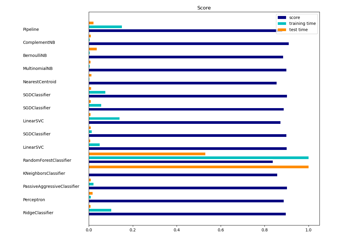
Classification of text documents using sparse features
======================================================

This is an example showing how scikit-learn can be used to classify documents
by topics using a bag-of-words approach. This example uses a scipy.sparse
matrix to store the features and demonstrates various classifiers that can
efficiently handle sparse matrices.

The dataset used in this example is the 20 newsgroups dataset. It will be
automatically downloaded, then cached.

"""

# Author: Peter Prettenhofer <peter.prettenhofer@gmail.com>
#         Olivier Grisel <olivier.grisel@ensta.org>
#         Mathieu Blondel <mathieu@mblondel.org>
#         Lars Buitinck
# License: BSD 3 clause
import logging
import numpy as np
from optparse import OptionParser
import sys
from time import time
import matplotlib.pyplot as plt

from sklearn.datasets import fetch_20newsgroups
from sklearn.feature_extraction.text import TfidfVectorizer
from sklearn.feature_extraction.text import HashingVectorizer
from sklearn.feature_selection import SelectFromModel
from sklearn.feature_selection import SelectKBest, chi2
from sklearn.linear_model import RidgeClassifier
from sklearn.pipeline import Pipeline
from sklearn.svm import LinearSVC
from sklearn.linear_model import SGDClassifier
from sklearn.linear_model import Perceptron
from sklearn.linear_model import PassiveAggressiveClassifier
from sklearn.naive_bayes import BernoulliNB, ComplementNB, MultinomialNB
from sklearn.neighbors import KNeighborsClassifier
from sklearn.neighbors import NearestCentroid
from sklearn.ensemble import RandomForestClassifier
from sklearn.utils.extmath import density
from sklearn import metrics


# Display progress logs on stdout
logging.basicConfig(level=logging.INFO,
                    format='%(asctime)s %(levelname)s %(message)s')

op = OptionParser()
op.add_option("--report",
              action="store_true", dest="print_report",
              help="Print a detailed classification report.")
op.add_option("--chi2_select",
              action="store", type="int", dest="select_chi2",
              help="Select some number of features using a chi-squared test")
op.add_option("--confusion_matrix",
              action="store_true", dest="print_cm",
              help="Print the confusion matrix.")
op.add_option("--top10",
              action="store_true", dest="print_top10",
              help="Print ten most discriminative terms per class"
                   " for every classifier.")
op.add_option("--all_categories",
              action="store_true", dest="all_categories",
              help="Whether to use all categories or not.")
op.add_option("--use_hashing",
              action="store_true",
              help="Use a hashing vectorizer.")
op.add_option("--n_features",
              action="store", type=int, default=2 ** 16,
              help="n_features when using the hashing vectorizer.")
op.add_option("--filtered",
              action="store_true",
              help="Remove newsgroup information that is easily overfit: "
                   "headers, signatures, and quoting.")


def is_interactive():
    return not hasattr(sys.modules['__main__'], '__file__')


# work-around for Jupyter notebook and IPython console
argv = [] if is_interactive() else sys.argv[1:]
(opts, args) = op.parse_args(argv)
if len(args) > 0:
    op.error("this script takes no arguments.")
    sys.exit(1)

print(__doc__)
op.print_help()
print()


# %%
# Load data from the training set
# ------------------------------------
# Let's load data from the newsgroups dataset which comprises around 18000
# newsgroups posts on 20 topics split in two subsets: one for training (or
# development) and the other one for testing (or for performance evaluation).
if opts.all_categories:
    categories = None
else:
    categories = [
        'alt.atheism',
        'talk.religion.misc',
        'comp.graphics',
        'sci.space',
    ]

if opts.filtered:
    remove = ('headers', 'footers', 'quotes')
else:
    remove = ()

print("Loading 20 newsgroups dataset for categories:")
print(categories if categories else "all")

data_train = fetch_20newsgroups(subset='train', categories=categories,
                                shuffle=True, random_state=42,
                                remove=remove)

data_test = fetch_20newsgroups(subset='test', categories=categories,
                               shuffle=True, random_state=42,
                               remove=remove)
print('data loaded')

# order of labels in `target_names` can be different from `categories`
target_names = data_train.target_names


def size_mb(docs):
    return sum(len(s.encode('utf-8')) for s in docs) / 1e6


data_train_size_mb = size_mb(data_train.data)
data_test_size_mb = size_mb(data_test.data)

print("%d documents - %0.3fMB (training set)" % (
    len(data_train.data), data_train_size_mb))
print("%d documents - %0.3fMB (test set)" % (
    len(data_test.data), data_test_size_mb))
print("%d categories" % len(target_names))
print()

# split a training set and a test set
y_train, y_test = data_train.target, data_test.target

print("Extracting features from the training data using a sparse vectorizer")
t0 = time()
if opts.use_hashing:
    vectorizer = HashingVectorizer(stop_words='english', alternate_sign=False,
                                   n_features=opts.n_features)
    X_train = vectorizer.transform(data_train.data)
else:
    vectorizer = TfidfVectorizer(sublinear_tf=True, max_df=0.5,
                                 stop_words='english')
    X_train = vectorizer.fit_transform(data_train.data)
duration = time() - t0
print("done in %fs at %0.3fMB/s" % (duration, data_train_size_mb / duration))
print("n_samples: %d, n_features: %d" % X_train.shape)
print()

print("Extracting features from the test data using the same vectorizer")
t0 = time()
X_test = vectorizer.transform(data_test.data)
duration = time() - t0
print("done in %fs at %0.3fMB/s" % (duration, data_test_size_mb / duration))
print("n_samples: %d, n_features: %d" % X_test.shape)
print()

# mapping from integer feature name to original token string
if opts.use_hashing:
    feature_names = None
else:
    feature_names = vectorizer.get_feature_names()

if opts.select_chi2:
    print("Extracting %d best features by a chi-squared test" %
          opts.select_chi2)
    t0 = time()
    ch2 = SelectKBest(chi2, k=opts.select_chi2)
    X_train = ch2.fit_transform(X_train, y_train)
    X_test = ch2.transform(X_test)
    if feature_names:
        # keep selected feature names
        feature_names = [feature_names[i] for i
                         in ch2.get_support(indices=True)]
    print("done in %fs" % (time() - t0))
    print()

if feature_names:
    feature_names = np.asarray(feature_names)


def trim(s):
    """Trim string to fit on terminal (assuming 80-column display)"""
    return s if len(s) <= 80 else s[:77] + "..."


# %%
# Benchmark classifiers
# ------------------------------------
# We train and test the datasets with 15 different classification models
# and get performance results for each model.
def benchmark(clf):
    print('_' * 80)
    print("Training: ")
    print(clf)
    t0 = time()
    clf.fit(X_train, y_train)
    train_time = time() - t0
    print("train time: %0.3fs" % train_time)

    t0 = time()
    pred = clf.predict(X_test)
    test_time = time() - t0
    print("test time:  %0.3fs" % test_time)

    score = metrics.accuracy_score(y_test, pred)
    print("accuracy:   %0.3f" % score)

    if hasattr(clf, 'coef_'):
        print("dimensionality: %d" % clf.coef_.shape[1])
        print("density: %f" % density(clf.coef_))

        if opts.print_top10 and feature_names is not None:
            print("top 10 keywords per class:")
            for i, label in enumerate(target_names):
                top10 = np.argsort(clf.coef_[i])[-10:]
                print(trim("%s: %s" % (label, " ".join(feature_names[top10]))))
        print()

    if opts.print_report:
        print("classification report:")
        print(metrics.classification_report(y_test, pred,
                                            target_names=target_names))

    if opts.print_cm:
        print("confusion matrix:")
        print(metrics.confusion_matrix(y_test, pred))

    print()
    clf_descr = str(clf).split('(')[0]
    return clf_descr, score, train_time, test_time


results = []
for clf, name in (
        (RidgeClassifier(tol=1e-2, solver="sag"), "Ridge Classifier"),
        (Perceptron(max_iter=50), "Perceptron"),
        (PassiveAggressiveClassifier(max_iter=50),
         "Passive-Aggressive"),
        (KNeighborsClassifier(n_neighbors=10), "kNN"),
        (RandomForestClassifier(), "Random forest")):
    print('=' * 80)
    print(name)
    results.append(benchmark(clf))

for penalty in ["l2", "l1"]:
    print('=' * 80)
    print("%s penalty" % penalty.upper())
    # Train Liblinear model
    results.append(benchmark(LinearSVC(penalty=penalty, dual=False,
                                       tol=1e-3)))

    # Train SGD model
    results.append(benchmark(SGDClassifier(alpha=.0001, max_iter=50,
                                           penalty=penalty)))

# Train SGD with Elastic Net penalty
print('=' * 80)
print("Elastic-Net penalty")
results.append(benchmark(SGDClassifier(alpha=.0001, max_iter=50,
                                       penalty="elasticnet")))

# Train NearestCentroid without threshold
print('=' * 80)
print("NearestCentroid (aka Rocchio classifier)")
results.append(benchmark(NearestCentroid()))

# Train sparse Naive Bayes classifiers
print('=' * 80)
print("Naive Bayes")
results.append(benchmark(MultinomialNB(alpha=.01)))
results.append(benchmark(BernoulliNB(alpha=.01)))
results.append(benchmark(ComplementNB(alpha=.1)))

print('=' * 80)
print("LinearSVC with L1-based feature selection")
# The smaller C, the stronger the regularization.
# The more regularization, the more sparsity.
results.append(benchmark(Pipeline([
  ('feature_selection', SelectFromModel(LinearSVC(penalty="l1", dual=False,
                                                  tol=1e-3))),
  ('classification', LinearSVC(penalty="l2"))])))


# %%
# Add plots
# ------------------------------------
# The bar plot indicates the accuracy, training time (normalized) and test time
# (normalized) of each classifier.
indices = np.arange(len(results))

results = [[x[i] for x in results] for i in range(4)]

clf_names, score, training_time, test_time = results
training_time = np.array(training_time) / np.max(training_time)
test_time = np.array(test_time) / np.max(test_time)

plt.figure(figsize=(12, 8))
plt.title("Score")
plt.barh(indices, score, .2, label="score", color='navy')
plt.barh(indices + .3, training_time, .2, label="training time",
         color='c')
plt.barh(indices + .6, test_time, .2, label="test time", color='darkorange')
plt.yticks(())
plt.legend(loc='best')
plt.subplots_adjust(left=.25)
plt.subplots_adjust(top=.95)
plt.subplots_adjust(bottom=.05)

for i, c in zip(indices, clf_names):
    plt.text(-.3, i, c)

plt.show()

Output

================================================================================
Ridge Classifier
________________________________________________________________________________
Training:
RidgeClassifier(solver='sag', tol=0.01)
/home/circleci/project/sklearn/linear_model/_ridge.py:555: UserWarning: "sag" solver requires many iterations to fit an intercept with sparse inputs. Either set the solver to "auto" or "sparse_cg", or set a low "tol" and a high "max_iter" (especially if inputs are not standardized).
  warnings.warn(
train time: 0.180s
test time:  0.001s
accuracy:   0.897
dimensionality: 33809
density: 1.000000


================================================================================
Perceptron
________________________________________________________________________________
Training:
Perceptron(max_iter=50)
train time: 0.017s
test time:  0.003s
accuracy:   0.888
dimensionality: 33809
density: 0.255302


================================================================================
Passive-Aggressive
________________________________________________________________________________
Training:
PassiveAggressiveClassifier(max_iter=50)
train time: 0.039s
test time:  0.002s
accuracy:   0.902
dimensionality: 33809
density: 0.692841


================================================================================
kNN
________________________________________________________________________________
Training:
KNeighborsClassifier(n_neighbors=10)
train time: 0.001s
test time:  0.171s
accuracy:   0.858

================================================================================
Random forest
________________________________________________________________________________
Training:
RandomForestClassifier()
train time: 1.765s
test time:  0.091s
accuracy:   0.837

================================================================================
L2 penalty
________________________________________________________________________________
Training:
LinearSVC(dual=False, tol=0.001)
train time: 0.088s
test time:  0.001s
accuracy:   0.900
dimensionality: 33809
density: 1.000000


________________________________________________________________________________
Training:
SGDClassifier(max_iter=50)
train time: 0.025s
test time:  0.002s
accuracy:   0.899
dimensionality: 33809
density: 0.569944


================================================================================
L1 penalty
________________________________________________________________________________
Training:
LinearSVC(dual=False, penalty='l1', tol=0.001)
train time: 0.247s
test time:  0.001s
accuracy:   0.873
dimensionality: 33809
density: 0.005561


________________________________________________________________________________
Training:
SGDClassifier(max_iter=50, penalty='l1')
train time: 0.099s
test time:  0.002s
accuracy:   0.888
dimensionality: 33809
density: 0.022982


================================================================================
Elastic-Net penalty
________________________________________________________________________________
Training:
SGDClassifier(max_iter=50, penalty='elasticnet')
train time: 0.132s
test time:  0.002s
accuracy:   0.902
dimensionality: 33809
density: 0.187502


================================================================================
NearestCentroid (aka Rocchio classifier)
________________________________________________________________________________
Training:
NearestCentroid()
train time: 0.004s
test time:  0.002s
accuracy:   0.855

================================================================================
Naive Bayes
________________________________________________________________________________
Training:
MultinomialNB(alpha=0.01)
train time: 0.008s
test time:  0.001s
accuracy:   0.899
/home/circleci/project/sklearn/utils/deprecation.py:101: FutureWarning: Attribute coef_ was deprecated in version 0.24 and will be removed in 1.1 (renaming of 0.26).
  warnings.warn(msg, category=FutureWarning)
dimensionality: 33809
density: 1.000000


________________________________________________________________________________
Training:
BernoulliNB(alpha=0.01)
train time: 0.008s
test time:  0.006s
accuracy:   0.884
/home/circleci/project/sklearn/utils/deprecation.py:101: FutureWarning: Attribute coef_ was deprecated in version 0.24 and will be removed in 1.1 (renaming of 0.26).
  warnings.warn(msg, category=FutureWarning)
dimensionality: 33809
density: 1.000000


________________________________________________________________________________
Training:
ComplementNB(alpha=0.1)
train time: 0.008s
test time:  0.002s
accuracy:   0.911
/home/circleci/project/sklearn/utils/deprecation.py:101: FutureWarning: Attribute coef_ was deprecated in version 0.24 and will be removed in 1.1 (renaming of 0.26).
  warnings.warn(msg, category=FutureWarning)
dimensionality: 33809
density: 1.000000


================================================================================
LinearSVC with L1-based feature selection
________________________________________________________________________________
Training:
Pipeline(steps=[('feature_selection',
                 SelectFromModel(estimator=LinearSVC(dual=False, penalty='l1',
                                                     tol=0.001))),
                ('classification', LinearSVC())])
train time: 0.265s
test time:  0.004s
accuracy:   0.880

SelectKBest

https://scikit-learn.org/stable/modules/generated/sklearn.feature_selection.SelectKBest.html

Select features according to the k highest scores.

See also

f_classif

ANOVA F-value between label/feature for classification tasks.

mutual_info_classif

Mutual information for a discrete target.

chi2

Chi-squared stats of non-negative features for classification tasks.

f_regression

F-value between label/feature for regression tasks.

mutual_info_regression

Mutual information for a continuous target.

SelectPercentile

Select features based on percentile of the highest scores.

SelectFpr

Select features based on a false positive rate test.

SelectFdr

Select features based on an estimated false discovery rate.

SelectFwe

Select features based on family-wise error rate.

GenericUnivariateSelect

Univariate feature selector with configurable mode.

>>> from sklearn.datasets import load_digits
>>> from sklearn.feature_selection import SelectKBest, chi2
>>> X, y = load_digits(return_X_y=True)
>>> X.shape
(1797, 64)
>>> X_new = SelectKBest(chi2, k=20).fit_transform(X, y)
>>> X_new.shape
(1797, 20)

Chi-squared test

对于一个null假设， 假设目标分布跟某一个特征没有显著差异。如果没有显著差异， 则词特征对目标没有更多的贡献，则可以考虑抛弃。

通过卡方检验判定，是否没有显著差异。

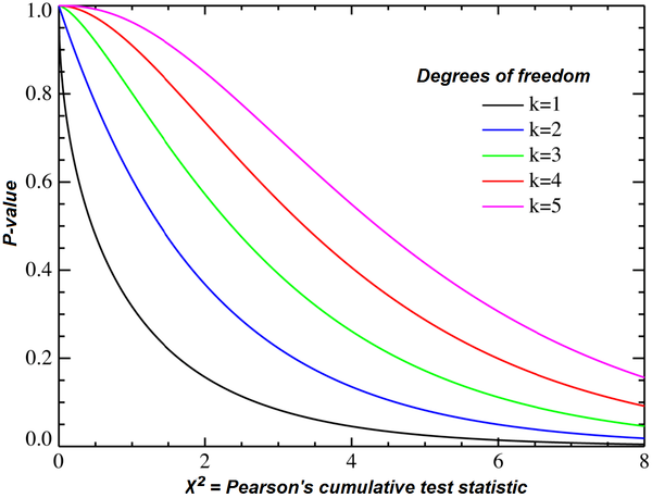
卡方检验， 通过计算卡方来查询p值， 重点是计算卡方值， 然后通过公式计算p值， 或者查表法查出p值。

p值越大， 表示null假设越是可信度高，则特征越是没有贡献， p表示possible。

p值越小， 越是需要关注其对目标的贡献度。

https://en.wikipedia.org/wiki/Chi-squared_test

A chi-squared test, also written as χ² test, is a statistical hypothesis test that is valid to perform when the test statistic is chi-squared distributed under the null hypothesis, specifically Pearson's chi-squared test and variants thereof. Pearson's chi-squared test is used to determine whether there is a statistically significant difference between the expected frequencies and the observed frequencies in one or more categories of a contingency table.

In the standard applications of this test, the observations are classified into mutually exclusive classes. If the null hypothesis that there are no differences between the classes in the population is true, the test statistic computed from the observations follows a χ² frequency distribution. The purpose of the test is to evaluate how likely the observed frequencies would be assuming the null hypothesis is true.

https://www.mathsisfun.com/data/chi-square-test.html

Example: "Which holiday do you prefer?"

	Beach	Cruise
Men	209	280
Women	225	248

Does Gender affect Preferred Holiday?

If Gender (Man or Woman) does affect Preferred Holiday we say they are dependent.

By doing some special calculations (explained later), we come up with a "p" value:

p value is 0.132

Now, p < 0.05 is the usual test for dependence.

In this case p is greater than 0.05, so we believe the variables are independent (ie not linked together).

In other words Men and Women probably do not have a different preference for Beach Holidays or Cruises.

It was just random differences which we expect when collecting data.

is_interactive

如何判断python是运行在命令行模式， 还是 交互式 运行模式？

只要判断__main__模块中是否包含 __file__ 变量即可。

命令行模式， 代码是从文件中加载进来， 所以有 __file__ 变量。

但是 交互模式， 其运行模式是 REPL ， 代码是从用户输入得到， 没有所谓的文件。

def is_interactive():
    return not hasattr(sys.modules['__main__'], '__file__')

INTERACTIVE MODE

The interactive mode of Python is also called REPL.

REPL stands for ‘Read-Eval-Print-Loop’. It is a simple, interactive command-line shell that provides us with the result when provided with a single line Python commands.

1. Read: The read function accepts an input from the user and stores it into the memory.
2. Eval: The eval function evaluates this ‘input’ read from the memory.
3. Print: The print function prints the outcome from the eval function.
4. Loop: The loop function creates a loop and terminates itself when the program ends.

This was a brief explanation of the interactive mode: REPL.

__file__

https://docs.python.org/3/reference/import.html#__file__

__file__ is optional. If set, this attribute’s value must be a string. The import system may opt to leave __file__ unset if it has no semantic meaning (e.g. a module loaded from a database).

If __file__ is set, it may also be appropriate to set the __cached__ attribute which is the path to any compiled version of the code (e.g. byte-compiled file). The file does not need to exist to set this attribute; the path can simply point to where the compiled file would exist (see PEP 3147).

It is also appropriate to set __cached__ when __file__ is not set. However, that scenario is quite atypical. Ultimately, the loader is what makes use of __file__ and/or __cached__. So if a loader can load from a cached module but otherwise does not load from a file, that atypical scenario may be appropriate.

https://stackoverflow.com/questions/28569328/python-main-file

When you run the script from a file then the __main__ module is in fact that file. In the Python interpreter prompt, on the other hand, the __main__ module is just the default namespace the interpreter, specifically the interactive prompt is running in, and it has no file associated with it (loosely speaking the file is <stdin>).

When you hit F5 to run the code in idle it's doing the equivalent to if you just copy/pasted that code into the interpreter directly. There is no way for it to have any association with that file.

If, on the other hand, you run import Test_ then now the code in that file is associated with the Test_ module and you'll find that Test_.__file__ gives the associated filename.

For what it's worth, there's almost never any reason to import __main__. If you want the script to print the file it was run out of you can just have:

if __name__ == '__main__':
    print __file__

among other possibilities.