R语言网络爬虫学习 基于rvest包

R语言网络爬虫学习 基于rvest包

龙君蛋君；2015年3月26日

1.背景介绍：

前几天看到有人写了一篇用R爬虫的文章，感兴趣，于是自己学习了。好吧，其实我和那篇文章R语言爬虫初尝试-基于RVEST包学习 的主人认识～

2.知识引用与学习：

1.R语言爬虫初尝试-基于RVEST包学习

2.大数据分析之——足彩数据趴取

3.rvest + CSS Selector 网页数据抓取的最佳选择

4.rvest的github

3.正文：

第一个爬虫是爬取了戴申大牛在科学网博客的一些基本信息，戴申大牛看到这篇文章不要打我啊～我只是爬取了博文的几个字段，求饶恕～

 

library(rvest)
library(sqldf)
library(gsubfn)
library(proto)
#creat a function
extrafun <- function(i,non_pn_url){
    url <- paste0(non_pn_url,i)
    web <- html(url)
    papername<- web %>% html_nodes("dl.bbda dt.xs2 a") %>% html_text()%>% .[c(seq(2,20,2))] %>% as.character()
    paperlink<-gsub("\\?source\\=search","",web %>% html_nodes("dl.bbda dt.xs2 a") %>% html_attr("href"))%>% .[c(seq(2,20,2))]
    paperlink <- paste0("http://blog.sciencenet.cn/",paperlink) %>% as.character()
    posttime <- web %>% html_nodes("dl.bbda dd span.xg1") %>% html_text() %>% as.Date()#这里取每篇文章的发布时间
    count_of_read <- web %>% html_nodes("dl.bbda dd.xg1 a") %>% html_text()
    count_of_read <- as.data.frame(count_of_read)
    count_of_read <- sqldf("select * from count_of_read where count_of_read like '%次阅读'")
    data.frame(papername,posttime,count_of_read,paperlink)
}
#crawl data
final <- data.frame()
url <- 'http://blog.sciencenet.cn/home.php?mod=space&uid=556556&do=blog&view=me&page='
for(i in 1:40){
   extrafun(i,url)
   final <- rbind(final,extrafun(i,url))
}
> dim(final)
[1] 400   4
> head(final)
                                                   papername
1                                             此均值非彼均值
2             [转载]孔丘、孔子、孔老二，它究竟是一只什么鸟？
3                          大数据分析之——k-means聚类中的坑
4                               大数据分析之——足彩数据趴取
5 [转载]老王这次要摊事了，当年他主管的部门是事被重新抖出来。
6                                 [转载]党卫军是这样抓人的。
    posttime count_of_read
1 2015-03-08    216 次阅读
2 2015-02-10    190 次阅读
3 2015-01-18    380 次阅读
4 2015-01-10    437 次阅读
5 2015-01-05    480 次阅读
6 2015-01-05    398 次阅读
                                          paperlink
1 http://blog.sciencenet.cn/blog-556556-872813.html
2 http://blog.sciencenet.cn/blog-556556-866932.html
3 http://blog.sciencenet.cn/blog-556556-860647.html
4 http://blog.sciencenet.cn/blog-556556-858171.html
5 http://blog.sciencenet.cn/blog-556556-856705.html
6 http://blog.sciencenet.cn/blog-556556-856640.html

抓取的数据不能直接用作分析，于是导出到Excel，对数据做了一些处理，然后绘制了一张图。

write.table(final,"final.csv",fileEncoding="GB2312")
#抓取的数据需要在Excel进一步加工，加工后读取进来，进一步做分析
a <- read.table("dai_shen_blog_0326.csv",header=TRUE,sep=";",fileEncoding="GB2312")#Mac OS 环境下，要sep＝";"
a$posttime <- as.Date(a$posttime)
a$paperlink <- as.character(a$paperlink)
a$papername <- as.character(a$papername)
a$count_of_read_NO. <- as.numeric(a$count_of_read_NO.)
library(ggplot2)
qplot(posttime,count_of_read_NO.,data=a,geom="point",colour=repost,size=6)

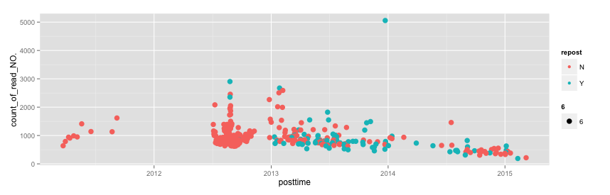
这张图说明了什么呢？？

a).戴大牛在2012年上半年没写文章也没有转载文章（不知道发生了什么，难道是忘记博客登录密码了，哈哈～有可能），但下半年原创文章数量是最多的，数量占life time约1/3；

b).在2013年一整年,文章数量上半年明显多余下半年，全年文章总数量占life time约2/5,且原创和转载各半；

c).在2014年中，上半年文章数量明显少于下半年，转载和原创各半。

第二个爬虫是爬取了NBA2014-2015常规赛技术统计排行 - 得分榜 

#Crawl NBA player statistics from sina
#web http://nba.sports.sina.com.cn/playerstats.php?s=0&e=49&key=1&t=1
library(rvest)
library(stringr)
library(sqldf)
rm(NBAdata)
start <- seq(0,250,50)
end <- seq(49,299,50)
getdata <- function(i){
    url <- paste0('http://nba.sports.sina.com.cn/playerstats.php?s=',start[i],'&e=',end[i],'&key=1&t=1')
    rank <- url %>% html_session() %>% html_nodes("table") %>% .[[2]] %>% html_nodes("td:nth-child(1)") %>% html_text()%>%.[-1]%>%as.numeric()
    player <- url %>% html_session() %>% html_nodes("table") %>% .[[2]] %>% html_nodes("td:nth-child(2)") %>% html_text()%>%.[-1]%>%str_sub(9,100)%>%as.character()
    team <- url %>% html_session() %>% html_nodes("table") %>% .[[2]] %>% html_nodes("td:nth-child(3)") %>% html_text()%>%.[-1]%>%str_sub(9,100)%>%as.character()
    avg_score <- url %>% html_session() %>% html_nodes("table") %>% .[[2]] %>% html_nodes("td:nth-child(4)") %>% html_text()%>%.[-1]
    total_score <- url %>% html_session() %>% html_nodes("table") %>% .[[2]] %>% html_nodes("td:nth-child(5)") %>% html_text()%>%.[-1]
    total_shoot <- url %>% html_session() %>% html_nodes("table") %>% .[[2]] %>% html_nodes("td:nth-child(6)") %>% html_text()%>%.[-1]
    three_point <- url %>% html_session() %>% html_nodes("table") %>% .[[2]] %>% html_nodes("td:nth-child(7)") %>% html_text()%>%.[-1]
    punish_point <- url %>% html_session() %>% html_nodes("table") %>% .[[2]] %>% html_nodes("td:nth-child(8)") %>% html_text()%>%.[-1]
    avg_time <- url %>% html_session() %>% html_nodes("table") %>% .[[2]] %>% html_nodes("td:nth-child(9)") %>% html_text()%>%.[-1]
    total_involve <- url %>% html_session() %>% html_nodes("table") %>% .[[2]] %>% html_nodes("td:nth-child(10)") %>% html_text()%>%.[-1]
    data.frame(rank,player,team,avg_score,total_score,total_shoot,three_point,punish_point,avg_time,total_involve)

}

NBAdata <- data.frame()
for(i in 1:6){
    NBAdata <- rbind(NBAdata,getdata(i))
}
NBAdata <- sqldf("select distinct * from NBAdata")
write.table(NBAdata,"NBAdata.csv",sep=",",fileEncoding="GB2312")

> head(NBAdata)
  rank            player team avg_score total_score
1    1 拉塞尔-威斯布鲁克 雷霆      27.3        1556
2    2       詹姆斯-哈登 火箭      27.1        1900
3    3     勒布朗-詹姆斯 骑士      25.8        1600
4    4     安东尼-戴维斯 鹈鹕      24.6        1403
5    5   德马库斯-考辛斯 国王      23.8        1308
6    6       斯蒂芬-库里 勇士      23.4        1618
  total_shoot three_point punish_point avg_time
1       42.7%       30.1%        84.6%     33.8
2         44%       36.8%        86.6%     36.8
3       49.2%       35.4%        71.9%     36.2
4       54.5%         10%        81.4%     36.2
5       46.5%       28.6%        80.2%     33.7
6       47.9%       42.2%        91.4%     32.9
  total_involve
1            57
2            70
3            62
4            57
5            55
6            69

发现NBA2014-2015常规赛技术统计排行 - 得分榜 有两个错误。

a).排名第50的NBA球星缺失。

b).数据有大量重复，初次爬取，有510条记录，最后发现原来这个数据统计本身就有很多重复，于是用SQL去重，得到270条记录。

4.总结：

a).SelectorGadget 真的很好用，但是貌似这个插件要FQ才能安装成功。SelectorGadget结合Google Chrome 使用，查找html_nodes 非常方便。

b).下次爬，要学尾巴同学，爬一些招聘网站的数据，给自己以后找工作做个参考嘛。

以上。

－－－－－－－－－－－－－－－－－－－－－－－－－－－－－－－－－－－－－－－－－－－－－－－－－－－－－－－－－－－－－－－－－－－－－－－－－－－－－－－－

以下内容修改于2015-04-01　

今天闲来无事，浏览戴申同学的一篇博文

http://blog.sciencenet.cn/blog-556556-848696.html

发现自己之前对于 NBA2014-2015常规赛技术统计排行 - 得分榜 这个爬虫写的极为失败，特做出以下更新：

library(rvest)
library(stringr)
library(sqldf)
start <- seq(0,250,50)
end <- seq(49,299,50)
getdata <- function(i){
    url <- paste0('http://nba.sports.sina.com.cn/playerstats.php?s=',start[i],'&e=',end[i],'&key=1&t=1')
    dat <- url %>% html() %>% html_nodes("table")%>%.[[2]]%>%html_table(head=TRUE)
    data.frame(dat)
}
NBAdata <- data.frame()
for(i in 1:6){
    NBAdata <- rbind(NBAdata,getdata(i))
}
NBAdata <- sqldf("select distinct * from NBAdata")
dim(NBAdata)
write.table(NBAdata,"NBAdata.csv",sep=",",fileEncoding="GB2312")

> head(NBAdata)
  排名              球员 球队 场均得分 得分总数 投篮命中率
1    1 拉塞尔-威斯布鲁克 雷霆     27.6     1626      42.5%
2    2       詹姆斯-哈登 火箭     27.2     1988      43.8%
3    3     勒布朗-詹姆斯 骑士     25.7     1644      48.9%
4    4     安东尼-戴维斯 鹈鹕     24.7     1455      54.1%
5    5   德马库斯-考辛斯 国王     24.1     1347      46.8%
6    6       斯蒂芬-库里 勇士     23.7     1708      48.3%
  三分命中率 罚篮命中率 场均时间 参赛场次
1      29.7%      84.6%     34.0       59
2      36.9%      86.6%     36.9       73
3      35.3%      71.7%     36.3       64
4        10%      81.2%     36.3       59
5      28.6%      79.7%     33.9       56
6      43.4%      91.8%     32.9       72

总结：网页中若有table，则可以直接读取，然后用html_table(),可以直接转化为table，十分方便。