本文介绍了Alex net 在imageNet Classification 中的惊人表现,获得了ImagaNet LSVRC2012第一的好成绩,开启了卷积神经网络在cv领域的广泛应用。
1.数据集
ImageNet [6], which consists of over 15 million labeled high-resolution images in over 22,000 categories.
here,ILSVRC uses a subset of ImageNet with roughly 1000 images in each of 1000 categories. In all, there are roughly 1.2 million training images, 50,000 validation images, and
150,000 testing images.我们在这从ImageNet 中生成一个1000类,每类大约1000张图片,即大约120万个训练样例,50000个验证样例,150,000个测试样例。
ImageNet consists of variable-resolution images, while our system requires a constant input dimensionality. Therefore, we down-sampled the images to a fixed resolution of 256 × 256. Given a
rectangular image, we first rescaled the image such that the shorter side was of length 256, and then cropped out the central 256×256 patch from the resulting image. We did not pre-process the images
in any other way, except for subtracting the mean activity over the training set from each pixel. So we trained our network on the (centered) raw RGB values of the pixels.
2.网络架构 The architecture of our network is summarized in Figure 2. It contains eight learned layers —five convolutional and three fully-connected
2.1 activation function
using RELU Nonlinearity,The standard way to model a neuron’s output f as
a function of its input x is with f (x) = tanh(x) or f (x) = (1 + e −x ) −1 . In terms of training time
with gradient descent, these saturating nonlinearities are much slower than the non-saturating nonlinearity f (x) = max(0, x).
Deep convolutional neural networks with ReLUs train several times faster than their equivalents with tanh units.
2.2 Training on Multiple GPUs
2.3 Local Response Normalization
2.4 Overlapping Pooling
Pooling layers in CNNs summarize the outputs of neighboring groups of neurons in the same kernel map. Traditionally, the neighborhoods summarized by adjacent pooling units do not overlap (e.g.,
[17, 11, 4]). To be more precise, a pooling layer can be thought of as consisting of a grid of pooling units spaced s pixels apart, each summarizing a neighborhood of size z × z centered at the location
of the pooling unit. If we set s = z, we obtain traditional local pooling as commonly employed in CNNs. If we set s < z, we obtain overlapping pooling. This is what we use throughout our
network, with s = 2 and z = 3. This scheme reduces the top-1 and top-5 error rates by 0.4% and 0.3%, respectively, as compared with the non-overlapping scheme s = 2, z = 2, which produces
output of equivalent dimensions. We generally observe during training that models with overlapping pooling find it slightly more difficult to overfit.
当池化窗口的大小为z*z时,如果stride<z ,则进行Overlapping pooling,如果stride=z ,则进行一般的池化操作
2.5 Overall Architectur
Now we are ready to describe the overall architecture of our CNN. As depicted in Figure 2, the net contains eight layers with weights; the first five are convolutional and the remaining three are fully-
connected. The output of the last fully-connected layer is fed to a 1000-way softmax which produces a distribution over the 1000 class labels. Our network maximizes the multinomial logistic regression
objective, which is equivalent to maximizing the average across training cases of the log-probability of the correct label under the prediction distribution. The kernels of the second, fourth, and fifth convolutional
layers are connected only to those kernel maps in the previous layer which reside on the same GPU (see Figure 2). The kernels of the third convolutional layer are connected to all kernel maps in the second layer.
The neurons in the fully-connected layers are connected to all neurons in the previous layer. Response-normalization layers follow the first and second convolutional layers. Max-pooling layers, of the kind described in Section
3.4, follow both response-normalization layers as well as the fifth convolutional layer. The ReLU non-linearity is applied to the output of every convolutional and fully-connected layer.
The first convolutional layer filters the 224 × 224 × 3 input image with 96 kernels of size 11 × 11 × 3with a stride of 4 pixels (this is the distance between the receptive field centers of neighboring
neurons in a kernel map). The second convolutional layer takes as input the (response-normalized and pooled) output of the first convolutional layer and filters it with 256 kernels of size 5 × 5 × 48.
The third, fourth, and fifth convolutional layers are connected to one another without any intervening pooling or normalization layers. The third convolutional layer has 384 kernels of size 3 × 3 ×
256 connected to the (normalized, pooled) outputs of the second convolutional layer. The fourth convolutional layer has 384 kernels of size 3 × 3 × 192 , and the fifth convolutional layer has 256
kernels of size 3 × 3 × 192. The fully-connected layers have 4096 neurons each.

3.降低overfitting
3.1 数据增广
The easiest and most common method to reduce overfitting on image data is to artificially enlarge the dataset using label-preserving transformations (e.g., [25, 4, 5]). We employ two distinct forms
of data augmentation, both of which allow transformed images to be produced from the original images with very little computation, so the transformed images do not need to be stored on disk.
In our implementation, the transformed images are generated in Python code on the CPU while the GPU is training on the previous batch of images. So these data augmentation schemes are, in effect,
computationally free.
The first form of data augmentation consists of generating image translations and horizontal reflections. We do this by extracting random 224 × 224 patches (and their horizontal reflections) from the
256×256 images and training our network on these extracted patches 4 . This increases the size of our training set by a factor of 2048, though the resulting training examples are, of course, highly inter-
dependent. Without this scheme, our network suffers from substantial overfitting, which would have forced us to use much smaller networks. At test time, the network makes a prediction by extracting
five 224 × 224 patches (the four corner patches and the center patch) as well as their horizontal reflections (hence ten patches in all), and averaging the predictions made by the network’s softmax
layer on the ten patches. The second form of data augmentation consists of altering the intensities of the RGB channels in training images. Specifically, we perform PCA on the set of RGB pixel values throughout the
ImageNet training set. To each training image, we add multiples of the found principal components,with magnitudes proportional to the corresponding eigenvalues times a random variable drawn from
a Gaussian with mean zero and standard deviation 0.1.
3.2 dropout
Combining the predictions of many different models is a very successful way to reduce test errors[1, 3], but it appears to be too expensive for big neural networks that already take several days
to train. There is, however, a very efficient version of model combination that only costs about a factor of two during training. The recently-introduced technique, called “dropout” [10], consists
of setting to zero the output of each hidden neuron with probability 0.5. The neurons which are “dropped out” in this way do not contribute to the forward pass and do not participate in back-
propagation. So every time an input is presented, the neural network samples a different architecture, but all these architectures share weights. This technique reduces complex co-adaptations of neurons,
since a neuron cannot rely on the presence of particular other neurons. It is, therefore, forced to
learn more robust features that are useful in conjunction with many different random subsets of the other neurons. At test time, we use all the neurons but multiply their outputs by 0.5, which is a
reasonable approximation to taking the geometric mean of the predictive distributions produced by the exponentially-many dropout networks.
We use dropout in the first two fully-connected layers of Figure 2. Without dropout, our network exhibits substantial overfitting. Dropout roughly doubles the number of iterations required to converge.
4. Learning details
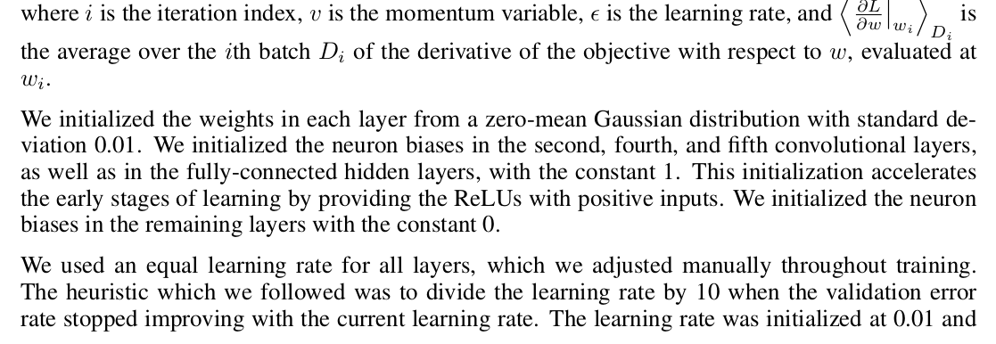
We trained our models using stochastic gradient descent with a batch size of 128 examples, momentum of 0.9, and
weight decay of 0.0005. We found that this small amount of weight decay was important for the model to learn. In
other words, weight decay here is not merely a regularizer: it reduces the model’s training error. The update rule for
weight w was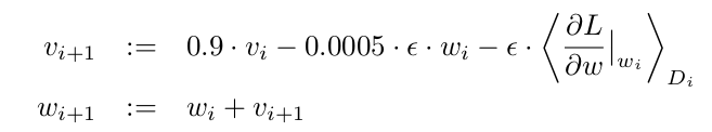
5 . Results