Python-根据成绩分析是否继续深造

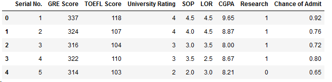
案例:该数据集的是一个关于每个学生成绩的数据集,接下来我们对该数据集进行分析，判断学生是否适合继续深造

数据集特征展示

    GRE 成绩 (290 to 340)
    TOEFL 成绩(92 to 120)
    学校等级 (1 to 5)
    自身的意愿 (1 to 5)
    推荐信的力度 (1 to 5)
    CGPA成绩 (6.8 to 9.92)
    是否有研习经验 (0 or 1)
    读硕士的意向 (0.34 to 0.97)

1.导入包

import numpy as np
import pandas as pd
import matplotlib.pyplot as plt
import seaborn as sns
import os,sys

2.导入并查看数据集

df = pd.read_csv("D:\machine-learning\score\Admission_Predict.csv",sep = ",")
print('There are ',len(df.columns),'columns')
for c in df.columns:
    sys.stdout.write(str(c)+', '

There are  9 columns
Serial No., GRE Score, TOEFL Score, University Rating, SOP, LOR , CGPA, Research, Chance of Admit , 
一共有9列特征

df.info()

<class 'pandas.core.frame.DataFrame'>
RangeIndex: 400 entries, 0 to 399
Data columns (total 9 columns):
Serial No.           400 non-null int64
GRE Score            400 non-null int64
TOEFL Score          400 non-null int64
University Rating    400 non-null int64
SOP                  400 non-null float64
LOR                  400 non-null float64
CGPA                 400 non-null float64
Research             400 non-null int64
Chance of Admit      400 non-null float64
dtypes: float64(4), int64(5)
memory usage: 28.2 KB

数据集信息：
　　1.数据有9个特征，分别是学号，GRE分数，托福分数，学校等级，SOP，LOR，CGPA，是否参加研习，进修的几率
　　2.数据集中没有空值
　　3.一共有400条数据

# 整理列名称
df = df.rename(columns={'Chance of Admit ':'Chance of Admit'})
# 显示前5列数据
df.head()

3.查看每个特征的相关性

fig,ax = plt.subplots(figsize=(10,10))
sns.heatmap(df.corr(),ax=ax,annot=True,linewidths=0.05,fmt='.2f',cmap='magma')
plt.show()

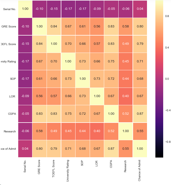
　　结论：1.最有可能影响是否读硕士的特征是GRE，CGPA，TOEFL成绩

　　　　　2.影响相对较小的特征是LOR，SOP，和Research

　4.数据可视化，双变量分析

　　　4.1 进行Research的人数

print("Not Having Research:",len(df[df.Research == 0]))
print("Having Research:",len(df[df.Research == 1]))
y = np.array([len(df[df.Research == 0]),len(df[df.Research == 1])])
x = np.arange(2)
plt.bar(x,y)
plt.title("Research Experience")
plt.xlabel("Canditates")
plt.ylabel("Frequency")
plt.xticks(x,('Not having research','Having research'))
plt.show()

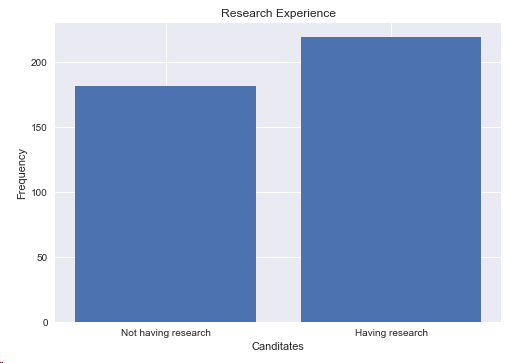
　　结论：进行research的人数是219，本科没有research人数是181

　　4.2 学生的托福成绩

y = np.array([df['TOEFL Score'].min(),df['TOEFL Score'].mean(),df['TOEFL Score'].max()])
x = np.arange(3)
plt.bar(x,y)
plt.title('TOEFL Score')
plt.xlabel('Level')
plt.ylabel('TOEFL Score')
plt.xticks(x,('Worst','Average','Best'))
plt.show()

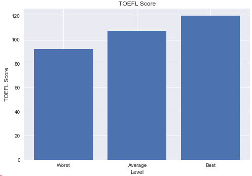
　　结论：最低分92分，最高分满分，进修学生的英语成绩很不错

　　4.3 GRE成绩

df['GRE Score'].plot(kind='hist',bins=200,figsize=(6,6))
plt.title('GRE Score')
plt.xlabel('GRE Score')
plt.ylabel('Frequency')
plt.show()

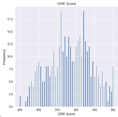
　　结论：310和330的分值的学生居多

　　4.4 CGPA和学校等级的关系

plt.scatter(df['University Rating'],df['CGPA'])
plt.title('CGPA Scores for University ratings')
plt.xlabel('University Rating')
plt.ylabel('CGPA')
plt.show()

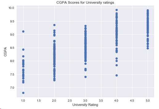
　　结论：学校越好，学生的GPA可能就越高

　　4.5 GRE成绩和CGPA的关系

plt.scatter(df['GRE Score'],df['CGPA'])
plt.title('CGPA for GRE Scores')
plt.xlabel('GRE Score')
plt.ylabel('CGPA')
plt.show()

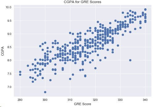
　　结论：GPA基点越高，GRE分数越高，2者的相关性很大

　　4.6 托福成绩和GRE成绩的关系

df[df['CGPA']>=8.5].plot(kind='scatter',x='GRE Score',y='TOEFL Score',color='red')
plt.xlabel('GRE Score')
plt.ylabel('TOEFL Score')
plt.title('CGPA >= 8.5')
plt.grid(True)
plt.show()

　　结论：多数情况下GRE和托福成正相关，但是GRE分数高，托福一定高。

　　4.6 学校等级和是否读硕士的关系

s = df[df['Chance of Admit'] >= 0.75]['University Rating'].value_counts().head(5)
plt.title('University Ratings of Candidates with an 75% acceptance chance')
s.plot(kind='bar',figsize=(20,10),cmap='Pastel1')
plt.xlabel('University Rating')
plt.ylabel('Candidates')
plt.show()

　　结论：排名靠前的学校的学生，进修的可能性更大

　　4.7 SOP和GPA的关系

plt.scatter(df['CGPA'],df['SOP'])
plt.xlabel('CGPA')
plt.ylabel('SOP')
plt.title('SOP for CGPA')
plt.show()

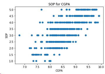
　　结论： GPA很高的学生，选择读硕士的自我意愿更强烈

　　4.8 SOP和GRE的关系

plt.scatter(df['GRE Score'],df['SOP'])
plt.xlabel('GRE Score')
plt.ylabel('SOP')
plt.title('SOP for GRE Score')
plt.show()

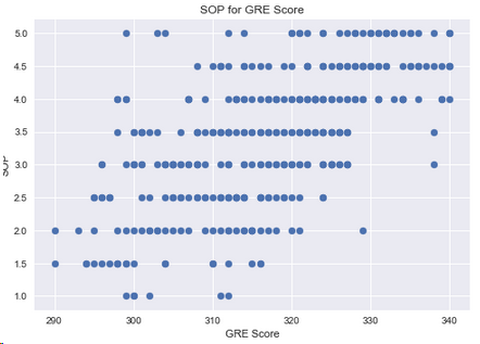
　　结论：读硕士意愿强的学生，GRE分数较高

5.模型

　　5.1 准备数据集

# 读取数据集
df = pd.read_csv('D:\machine-learning\score\Admission_Predict.csv',sep=',')

serialNO = df['Serial No.'].values

df.drop(['Serial No.'],axis=1,inplace=True)
df = df.rename(columns={'Chance of Admit ':'Chance of Admit'})

# 分割数据集
y = df['Chance of Admit'].values
x = df.drop(['Chance of Admit'],axis=1)

from sklearn.model_selection import train_test_split
x_train,x_test,y_train,y_test = train_test_split(x,y,test_size=0.2,random_state=42)

# 归一化数据
from sklearn.preprocessing import MinMaxScaler
scaleX = MinMaxScaler(feature_range=[0,1])
x_train[x_train.columns] = scaleX.fit_transform(x_train[x_train.columns])
x_test[x_test.columns] = scaleX.fit_transform(x_test[x_test.columns])

　　5.2 回归

　　　　5.2.1 线性回归

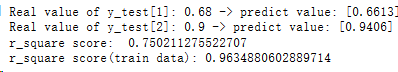
from sklearn.linear_model import LinearRegression

lr = LinearRegression()
lr.fit(x_train,y_train)
y_head_lr = lr.predict(x_test)

print('Real value of y_test[1]: '+str(y_test[1]) + ' -> predict value: ' + str(lr.predict(x_test.iloc[[1],:])))
print('Real value of y_test[2]: '+str(y_test[2]) + ' -> predict value: ' + str(lr.predict(x_test.iloc[[2],:])))

from sklearn.metrics import r2_score
print('r_square score: ',r2_score(y_test,y_head_lr))
y_head_lr_train = lr.predict(x_train)
print('r_square score(train data):',r2_score(y_train,y_head_lr_train))

　　　　5.2.2 随机森林回归

from sklearn.ensemble import RandomForestRegressor

rfr = RandomForestRegressor(n_estimators=100,random_state=42)
rfr.fit(x_train,y_train)
y_head_rfr = rfr.predict(x_test)

print('Real value of y_test[1]: '+str(y_test[1]) + ' -> predict value: ' + str(rfr.predict(x_test.iloc[[1],:])))
print('Real value of y_test[2]: '+str(y_test[2]) + ' -> predict value: ' + str(rfr.predict(x_test.iloc[[2],:])))

from sklearn.metrics import r2_score
print('r_square score: ',r2_score(y_test,y_head_rfr))
y_head_rfr_train = rfr.predict(x_train)
print('r_square score(train data):',r2_score(y_train,y_head_rfr_train))

　　　　5.2.3 决策树回归

from sklearn.tree import DecisionTreeRegressor

dt = DecisionTreeRegressor(random_state=42)
dt.fit(x_train,y_train)
y_head_dt = dt.predict(x_test)

print('Real value of y_test[1]: '+str(y_test[1]) + ' -> predict value: ' + str(dt.predict(x_test.iloc[[1],:])))
print('Real value of y_test[2]: '+str(y_test[2]) + ' -> predict value: ' + str(dt.predict(x_test.iloc[[2],:])))

from sklearn.metrics import r2_score
print('r_square score: ',r2_score(y_test,y_head_dt))
y_head_dt_train = dt.predict(x_train)
print('r_square score(train data):',r2_score(y_train,y_head_dt_train))

　　　　5.2.4 三种回归方法比较

y = np.array([r2_score(y_test,y_head_lr),r2_score(y_test,y_head_rfr),r2_score(y_test,y_head_dt)])
x = np.arange(3)
plt.bar(x,y)
plt.title('Comparion of Regression Algorithms')
plt.xlabel('Regression')
plt.ylabel('r2_score')
plt.xticks(x,("LinearRegression","RandomForestReg.","DecisionTreeReg."))
plt.show()

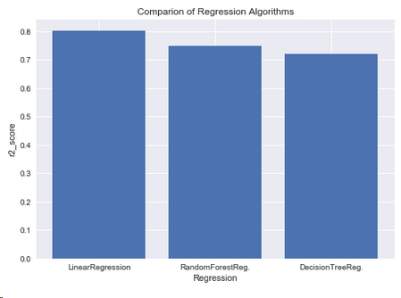
　　　　结论 ： 回归算法中，线性回归的性能更优

　　　　5.2.5 三种回归方法与实际值的比较

​red = plt.scatter(np.arange(0,80,5),y_head_lr[0:80:5],color='red')
blue = plt.scatter(np.arange(0,80,5),y_head_rfr[0:80:5],color='blue')
green = plt.scatter(np.arange(0,80,5),y_head_dt[0:80:5],color='green')
black = plt.scatter(np.arange(0,80,5),y_test[0:80:5],color='black')
plt.title('Comparison of Regression Algorithms')
plt.xlabel('Index of candidate')
plt.ylabel('Chance of admit')
plt.legend([red,blue,green,black],['LR','RFR','DT','REAL'])
plt.show()

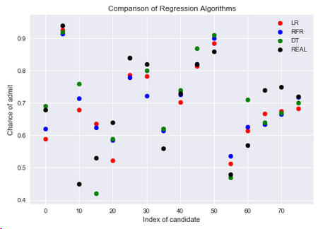
　　　　结论：在数据集中有70%的候选人有可能读硕士，从上图来看还有些点没有很好的得到预测

　　5.3 分类算法

　　　　5.3.1 准备数据

df = pd.read_csv('D:\machine-learning\score\Admission_Predict.csv',sep=',')

SerialNO = df['Serial No.'].values
df.drop(['Serial No.'],axis=1,inplace=True)

df = df.rename(columns={'Chance of Admit ':'Chance of Admit'})
y = df['Chance of Admit'].values
x = df.drop(['Chance of Admit'],axis=1)


from sklearn.model_selection import train_test_split
x_train,x_test,y_train,y_test = train_test_split(x,y,test_size=0.2,random_state=42)

from sklearn.preprocessing import MinMaxScaler
scaleX = MinMaxScaler(feature_range=[0,1])
x_train[x_train.columns] = scaleX.fit_transform(x_train[x_train.columns])
x_test[x_test.columns] = scaleX.fit_transform(x_test[x_test.columns])

# 如果chance >0.8, chance of admit 就是1，否则就是0
y_train_01 = [1 if each > 0.8 else 0 for each in y_train]
y_test_01 = [1 if each > 0.8 else 0 for each in y_test]

y_train_01 = np.array(y_train_01)
y_test_01 = np.array(y_test_01)

　　　　5.3.2 逻辑回归

from sklearn.linear_model import LogisticRegression

lrc = LogisticRegression()
lrc.fit(x_train,y_train_01)
print('score: ',lrc.score(x_test,y_test_01))
print('Real value of y_test_01[1]: '+str(y_test_01[1]) + ' -> predict value: ' + str(lrc.predict(x_test.iloc[[1],:])))
print('Real value of y_test_01[2]: '+str(y_test_01[2]) + ' -> predict value: ' + str(lrc.predict(x_test.iloc[[2],:])))

from sklearn.metrics import confusion_matrix
cm_lrc = confusion_matrix(y_test_01,lrc.predict(x_test))

f,ax = plt.subplots(figsize=(5,5))
sns.heatmap(cm_lrc,annot=True,linewidths=0.5,linecolor='red',fmt='.0f',ax=ax)
plt.title('Test for Test dataset')
plt.xlabel('predicted y values')
plt.ylabel('real y value')
plt.show()

from sklearn.metrics import recall_score,precision_score,f1_score
print('precision_score is : ',precision_score(y_test_01,lrc.predict(x_test)))
print('recall_score is : ',recall_score(y_test_01,lrc.predict(x_test)))
print('f1_score is : ',f1_score(y_test_01,lrc.predict(x_test)))

# Test for Train Dataset:

cm_lrc_train = confusion_matrix(y_train_01,lrc.predict(x_train))
f,ax = plt.subplots(figsize=(5,5))
sns.heatmap(cm_lrc_train,annot=True,linewidths=0.5,linecolor='blue',fmt='.0f',ax=ax)
plt.title('Test for Train dataset')
plt.xlabel('predicted y values')
plt.ylabel('real y value')
plt.show()

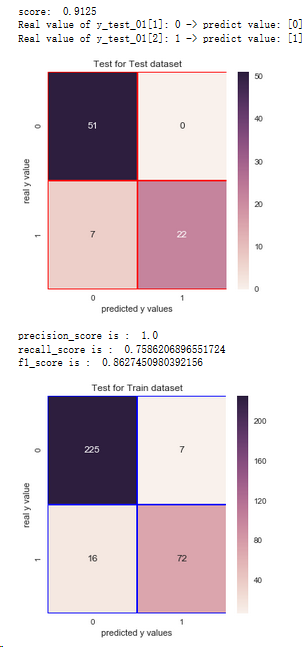
　　　　结论：1.通过混淆矩阵，逻辑回归算法在训练集样本上，有23个分错的样本，有72人想进一步读硕士

　　　　　　　2.在测试集上有7个分错的样本　

　　　　5.3.3 支持向量机（SVM）

from sklearn.svm import SVC

svm = SVC(random_state=1,kernel='rbf')
svm.fit(x_train,y_train_01)
print('score: ',svm.score(x_test,y_test_01))
print('Real value of y_test_01[1]: '+str(y_test_01[1]) + ' -> predict value: ' + str(svm.predict(x_test.iloc[[1],:])))
print('Real value of y_test_01[2]: '+str(y_test_01[2]) + ' -> predict value: ' + str(svm.predict(x_test.iloc[[2],:])))

from sklearn.metrics import confusion_matrix
cm_svm = confusion_matrix(y_test_01,svm.predict(x_test))

f,ax = plt.subplots(figsize=(5,5))
sns.heatmap(cm_svm,annot=True,linewidths=0.5,linecolor='red',fmt='.0f',ax=ax)
plt.title('Test for Test dataset')
plt.xlabel('predicted y values')
plt.ylabel('real y value')
plt.show()

from sklearn.metrics import recall_score,precision_score,f1_score
print('precision_score is : ',precision_score(y_test_01,svm.predict(x_test)))
print('recall_score is : ',recall_score(y_test_01,svm.predict(x_test)))
print('f1_score is : ',f1_score(y_test_01,svm.predict(x_test)))

# Test for Train Dataset:

cm_svm_train = confusion_matrix(y_train_01,svm.predict(x_train))
f,ax = plt.subplots(figsize=(5,5))
sns.heatmap(cm_svm_train,annot=True,linewidths=0.5,linecolor='blue',fmt='.0f',ax=ax)
plt.title('Test for Train dataset')
plt.xlabel('predicted y values')
plt.ylabel('real y value')
plt.show()

　

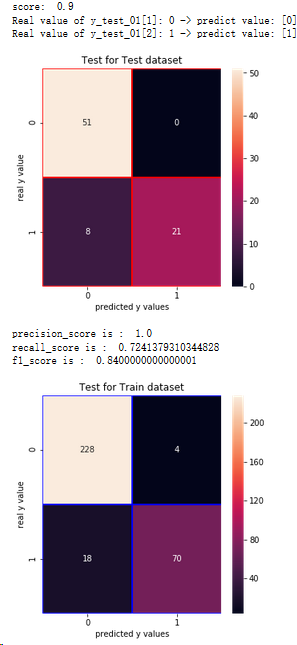
　　　　结论：1.通过混淆矩阵，SVM算法在训练集样本上，有22个分错的样本，有70人想进一步读硕士

　　　　　　　2.在测试集上有8个分错的样本

　　　　5.3.4 朴素贝叶斯

from sklearn.naive_bayes import GaussianNB

nb = GaussianNB()
nb.fit(x_train,y_train_01)
print('score: ',nb.score(x_test,y_test_01))
print('Real value of y_test_01[1]: '+str(y_test_01[1]) + ' -> predict value: ' + str(nb.predict(x_test.iloc[[1],:])))
print('Real value of y_test_01[2]: '+str(y_test_01[2]) + ' -> predict value: ' + str(nb.predict(x_test.iloc[[2],:])))

from sklearn.metrics import confusion_matrix
cm_nb = confusion_matrix(y_test_01,nb.predict(x_test))

f,ax = plt.subplots(figsize=(5,5))
sns.heatmap(cm_nb,annot=True,linewidths=0.5,linecolor='red',fmt='.0f',ax=ax)
plt.title('Test for Test dataset')
plt.xlabel('predicted y values')
plt.ylabel('real y value')
plt.show()

from sklearn.metrics import recall_score,precision_score,f1_score
print('precision_score is : ',precision_score(y_test_01,nb.predict(x_test)))
print('recall_score is : ',recall_score(y_test_01,nb.predict(x_test)))
print('f1_score is : ',f1_score(y_test_01,nb.predict(x_test)))

# Test for Train Dataset:

cm_nb_train = confusion_matrix(y_train_01,nb.predict(x_train))
f,ax = plt.subplots(figsize=(5,5))
sns.heatmap(cm_nb_train,annot=True,linewidths=0.5,linecolor='blue',fmt='.0f',ax=ax)
plt.title('Test for Train dataset')
plt.xlabel('predicted y values')
plt.ylabel('real y value')
plt.show()

　　  结论：1.通过混淆矩阵，朴素贝叶斯算法在训练集样本上，有20个分错的样本，有78人想进一步读硕士

　　　　　  2.在测试集上有7个分错的样本

　　　　5.3.5 随机森林分类器

from sklearn.ensemble import RandomForestClassifier

rfc = RandomForestClassifier(n_estimators=100,random_state=1)
rfc.fit(x_train,y_train_01)
print('score: ',rfc.score(x_test,y_test_01))
print('Real value of y_test_01[1]: '+str(y_test_01[1]) + ' -> predict value: ' + str(rfc.predict(x_test.iloc[[1],:])))
print('Real value of y_test_01[2]: '+str(y_test_01[2]) + ' -> predict value: ' + str(rfc.predict(x_test.iloc[[2],:])))

from sklearn.metrics import confusion_matrix
cm_rfc = confusion_matrix(y_test_01,rfc.predict(x_test))

f,ax = plt.subplots(figsize=(5,5))
sns.heatmap(cm_rfc,annot=True,linewidths=0.5,linecolor='red',fmt='.0f',ax=ax)
plt.title('Test for Test dataset')
plt.xlabel('predicted y values')
plt.ylabel('real y value')
plt.show()

from sklearn.metrics import recall_score,precision_score,f1_score
print('precision_score is : ',precision_score(y_test_01,rfc.predict(x_test)))
print('recall_score is : ',recall_score(y_test_01,rfc.predict(x_test)))
print('f1_score is : ',f1_score(y_test_01,rfc.predict(x_test)))

# Test for Train Dataset:

cm_rfc_train = confusion_matrix(y_train_01,rfc.predict(x_train))
f,ax = plt.subplots(figsize=(5,5))
sns.heatmap(cm_rfc_train,annot=True,linewidths=0.5,linecolor='blue',fmt='.0f',ax=ax)
plt.title('Test for Train dataset')
plt.xlabel('predicted y values')
plt.ylabel('real y value')
plt.show()

　　   结论：1.通过混淆矩阵，随机森林算法在训练集样本上，有0个分错的样本，有88人想进一步读硕士

　　　　　   2.在测试集上有5个分错的样本

　　　　5.3.6 决策树分类器

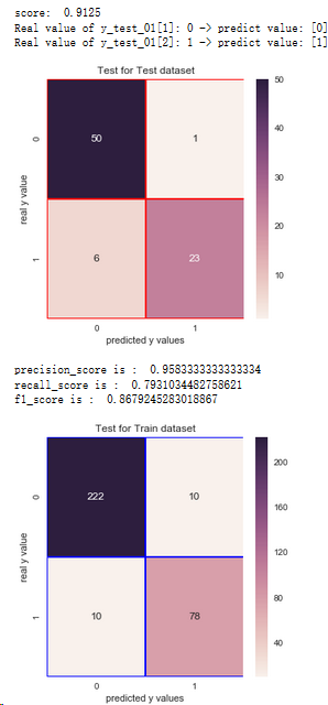
from sklearn.tree import DecisionTreeClassifier

dtc = DecisionTreeClassifier(criterion='entropy',max_depth=3)
dtc.fit(x_train,y_train_01)
print('score: ',dtc.score(x_test,y_test_01))
print('Real value of y_test_01[1]: '+str(y_test_01[1]) + ' -> predict value: ' + str(dtc.predict(x_test.iloc[[1],:])))
print('Real value of y_test_01[2]: '+str(y_test_01[2]) + ' -> predict value: ' + str(dtc.predict(x_test.iloc[[2],:])))

from sklearn.metrics import confusion_matrix
cm_dtc = confusion_matrix(y_test_01,dtc.predict(x_test))

f,ax = plt.subplots(figsize=(5,5))
sns.heatmap(cm_dtc,annot=True,linewidths=0.5,linecolor='red',fmt='.0f',ax=ax)
plt.title('Test for Test dataset')
plt.xlabel('predicted y values')
plt.ylabel('real y value')
plt.show()

from sklearn.metrics import recall_score,precision_score,f1_score
print('precision_score is : ',precision_score(y_test_01,dtc.predict(x_test)))
print('recall_score is : ',recall_score(y_test_01,dtc.predict(x_test)))
print('f1_score is : ',f1_score(y_test_01,dtc.predict(x_test)))

# Test for Train Dataset:

cm_dtc_train = confusion_matrix(y_train_01,dtc.predict(x_train))
f,ax = plt.subplots(figsize=(5,5))
sns.heatmap(cm_dtc_train,annot=True,linewidths=0.5,linecolor='blue',fmt='.0f',ax=ax)
plt.title('Test for Train dataset')
plt.xlabel('predicted y values')
plt.ylabel('real y value')
plt.show()

　　  结论：1.通过混淆矩阵，决策树算法在训练集样本上，有20个分错的样本，有78人想进一步读硕士

　　　　　   2.在测试集上有7个分错的样本

　　　　5.3.7 K临近分类器

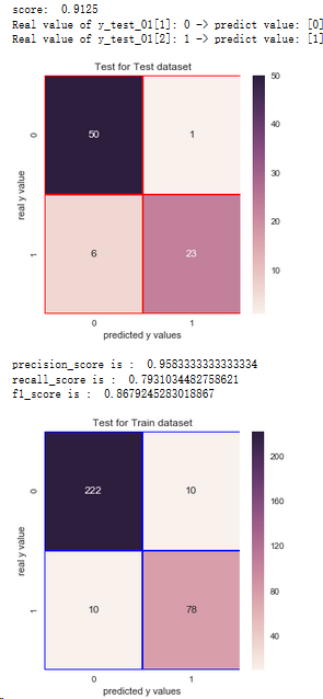
from sklearn.neighbors import KNeighborsClassifier

scores = []
for each in range(1,50):
    knn_n = KNeighborsClassifier(n_neighbors = each)
    knn_n.fit(x_train,y_train_01)
    scores.append(knn_n.score(x_test,y_test_01))
    
plt.plot(range(1,50),scores)
plt.xlabel('k')
plt.ylabel('Accuracy')
plt.show()


knn = KNeighborsClassifier(n_neighbors=7)
knn.fit(x_train,y_train_01)
print('score 7 : ',knn.score(x_test,y_test_01))
print('Real value of y_test_01[1]: '+str(y_test_01[1]) + ' -> predict value: ' + str(knn.predict(x_test.iloc[[1],:])))
print('Real value of y_test_01[2]: '+str(y_test_01[2]) + ' -> predict value: ' + str(knn.predict(x_test.iloc[[2],:])))

from sklearn.metrics import confusion_matrix
cm_knn = confusion_matrix(y_test_01,knn.predict(x_test))

f,ax = plt.subplots(figsize=(5,5))
sns.heatmap(cm_knn,annot=True,linewidths=0.5,linecolor='red',fmt='.0f',ax=ax)
plt.title('Test for Test dataset')
plt.xlabel('predicted y values')
plt.ylabel('real y value')
plt.show()

from sklearn.metrics import recall_score,precision_score,f1_score
print('precision_score is : ',precision_score(y_test_01,knn.predict(x_test)))
print('recall_score is : ',recall_score(y_test_01,knn.predict(x_test)))
print('f1_score is : ',f1_score(y_test_01,knn.predict(x_test)))

# Test for Train Dataset:

cm_knn_train = confusion_matrix(y_train_01,knn.predict(x_train))
f,ax = plt.subplots(figsize=(5,5))
sns.heatmap(cm_knn_train,annot=True,linewidths=0.5,linecolor='blue',fmt='.0f',ax=ax)
plt.title('Test for Train dataset')
plt.xlabel('predicted y values')
plt.ylabel('real y value')
plt.show()

　　　 结论：1.通过混淆矩阵，K临近算法在训练集样本上，有22个分错的样本，有71人想进一步读硕士

　　　　　   2.在测试集上有7个分错的样本

　　　5.3.8 分类器比较

y = np.array([lrc.score(x_test,y_test_01),svm.score(x_test,y_test_01),nb.score(x_test,y_test_01),
              dtc.score(x_test,y_test_01),rfc.score(x_test,y_test_01),knn.score(x_test,y_test_01)])
x = np.arange(6)
plt.bar(x,y)
plt.title('Comparison of Classification Algorithms')
plt.xlabel('Classification')
plt.ylabel('Score')
plt.xticks(x,("LogisticReg.","SVM","GNB","Dec.Tree","Ran.Forest","KNN"))
plt.show()

　　　　　

　　　　结论：随机森林和朴素贝叶斯二者的预测值都比较高

　　5.4 聚类算法

　　　　5.4.1 准备数据

df = pd.read_csv('D:\machine-learning\score\Admission_Predict.csv',sep=',')
df = df.rename(columns={'Chance of Admit ':'Chance of Admit'})
serialNo = df['Serial No.']
df.drop(['Serial No.'],axis=1,inplace=True)
df = (df - np.min(df)) / (np.max(df)-np.min(df))
y = df['Chance of Admit']
x = df.drop(['Chance of Admit'],axis=1)

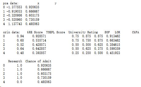
　　     5.4.2 降维

from sklearn.decomposition import PCA

pca = PCA(n_components=1,whiten=True)
pca.fit(x)
x_pca = pca.transform(x)
x_pca = x_pca.reshape(400)
dictionary = {'x':x_pca,'y':y}
data = pd.DataFrame(dictionary)
print('pca data:',data.head())

print()

print('orin data:',df.head())

　　　　5.4.3 K均值聚类

from sklearn.cluster import KMeans

wcss = []
for k in range(1,15):
    kmeans = KMeans(n_clusters=k)
    kmeans.fit(x)
    wcss.append(kmeans.inertia_)
plt.plot(range(1,15),wcss)
plt.xlabel('Kmeans')
plt.ylabel('WCSS')
plt.show()

df["Serial No."] = serialNo
kmeans = KMeans(n_clusters=3)
clusters_knn = kmeans.fit_predict(x)
df['label_kmeans'] = clusters_knn


plt.scatter(df[df.label_kmeans == 0 ]["Serial No."],df[df.label_kmeans == 0]['Chance of Admit'],color = "red")
plt.scatter(df[df.label_kmeans == 1 ]["Serial No."],df[df.label_kmeans == 1]['Chance of Admit'],color = "blue")
plt.scatter(df[df.label_kmeans == 2 ]["Serial No."],df[df.label_kmeans == 2]['Chance of Admit'],color = "green")
plt.title("K-means Clustering")
plt.xlabel("Candidates")
plt.ylabel("Chance of Admit")
plt.show()

plt.scatter(data.x[df.label_kmeans == 0 ],data[df.label_kmeans == 0].y,color = "red")
plt.scatter(data.x[df.label_kmeans == 1 ],data[df.label_kmeans == 1].y,color = "blue")
plt.scatter(data.x[df.label_kmeans == 2 ],data[df.label_kmeans == 2].y,color = "green")
plt.title("K-means Clustering")
plt.xlabel("X")
plt.ylabel("Chance of Admit")
plt.show()

　　

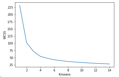
　　　　结论：数据集分成三个类别，一部分学生是决定继续读硕士，一部分放弃，还有一部分学生的比较犹豫，但是深造的可能性较大

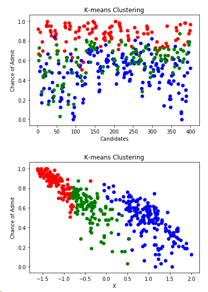
　　　　5.4.4 层次聚类

from scipy.cluster.hierarchy import linkage,dendrogram

merg = linkage(x,method='ward')
dendrogram(merg,leaf_rotation=90)
plt.xlabel('data points')
plt.ylabel('euclidean distance')
plt.show()

from sklearn.cluster import AgglomerativeClustering

hiyerartical_cluster = AgglomerativeClustering(n_clusters=3,affinity='euclidean',linkage='ward')
clusters_hiyerartical = hiyerartical_cluster.fit_predict(x)
df['label_hiyerartical'] = clusters_hiyerartical

plt.scatter(df[df.label_hiyerartical == 0 ]["Serial No."],df[df.label_hiyerartical == 0]['Chance of Admit'],color = "red")
plt.scatter(df[df.label_hiyerartical == 1 ]["Serial No."],df[df.label_hiyerartical == 1]['Chance of Admit'],color = "blue")
plt.scatter(df[df.label_hiyerartical == 2 ]["Serial No."],df[df.label_hiyerartical == 2]['Chance of Admit'],color = "green")
plt.title('Hierarchical Clustering')
plt.xlabel('Candidates')
plt.ylabel('Chance of Admit')
plt.show()

plt.scatter(data[df.label_hiyerartical == 0].x,data.y[df.label_hiyerartical==0],color='red')
plt.scatter(data[df.label_hiyerartical == 1].x,data.y[df.label_hiyerartical==1],color='blue')
plt.scatter(data[df.label_hiyerartical == 2].x,data.y[df.label_hiyerartical==2],color='green')
plt.title('Hierarchical Clustering')
plt.xlabel('X')
plt.ylabel('Chance of Admit')
plt.show()

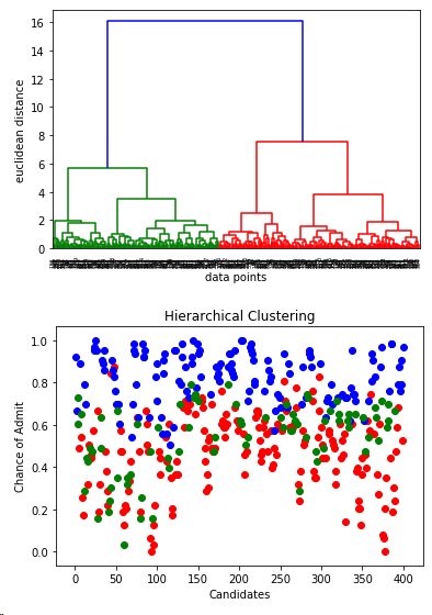
　　　　结论：从层次聚类的结果中，可以看出和K均值聚类的结果一致，只不过确定了聚类k的取值3

结论：通过本词入门数据集的训练，可以掌握

　　   1.一些特征的展示的方法

          2.如何调用sklearn 的API

          3.如何取比较不同模型之间的好坏

代码+数据集：https://github.com/Mounment/python-data-analyze/tree/master/kaggle/score

如果有用的话，记得打一个星星，谢谢