案例:员工流失是困扰企业的关键因素之一,在这次的分析中我将分析以下内容:
对一些重要变量进行可视化及探索分析,收入,晋升,满意度,绩效,是否加班等方面进行单变量分析
分析员工流失的因素,探索各个变量的影响度
构建有效的模型来预测员工是否会离职
数据集主要分析的字段
## Attrition 是否离职    需要预测的结果变量
## Gender 性别
## Age 年龄
## Education 学历
## NumCompaniesWorked 任职过的企业数量
## TotalWorkingYears 工作年限
## MaritalStatus 婚姻状况
## YearsAtCompany 在公司的工作时间
## JobRole 职位
## JobLevel 职位等级
## MonthlyIncome 月薪
## JobInvolvement 工作投入程度
## PerformanceRating 绩效评分
## StockOptionLevel 员工的股权等级
## PercentSalaryHike 涨薪百分比
## TrainingTimesLastYear 上一年培训次数
## YearsSinceLastPromotion 距离上次升值的时间
## EnvironmentSatisfaction 环境满意度
## JobSatisfaction 工作满意度
## RelationshipSatisfaction 关系满意度
## WorkLifeBalance 生活和工作的平衡度
## DistanceFromHome 公司和家庭的距离
## OverTime 是否要加班
## BusinessTravel 是否要出差
1.导入包
library(ggplot2)
library(grid)
library(gridExtra)
library(plyr)
library(rpart)
library(rpart.plot)
library(randomForest)
library(caret)
library(gbm)
library(survival)
library(pROC)
library(DMwR)
library(scales)
2.导入数据集并查看
Attr.df <- read.csv('E:\Udacity\Data Analysis High\R\R_Study\employee.csv',header=T,encoding = 'UTF-8')
head(Attr.df)
summary(Attr.df)
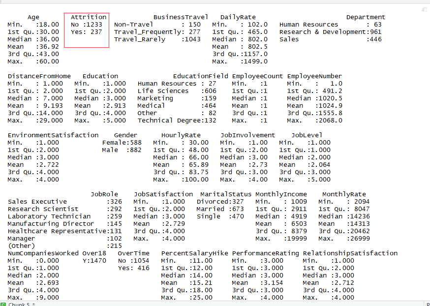
结论:离职率大概在1:5左右
企业的员工的平均年龄在36,37岁左右
月薪的大概是在4900美元,这里采用中位数,平均数会引起偏差
3.单变量分析
3.1探索性别,年龄,工龄,企业数量,在公司的时限的分析
# 离职员工年龄的分布
g1 <- ggplot(Attr.df,aes(x=Age,fill=Attrition))+
  geom_density(alpha=0.7)

# 离职员工工作过的企业数量的关系
g2 <- ggplot(Attr.df,aes(x=NumCompaniesWorked,fill=Attrition))+
  geom_density(alpha=0.7)

# 离职员工工龄的分布
g3 <- ggplot(Attr.df,aes(x=YearsAtCompany,fill=Attrition))+
  geom_density(alpha=0.7)

# 离职员工总体工作年限的分布
g4 <- ggplot(Attr.df,aes(x=TotalWorkingYears,fill=Attrition))+
  geom_density(alpha=0.7)
grid.arrange(g1,g2,g3,g4,ncol=2,nrow=2)
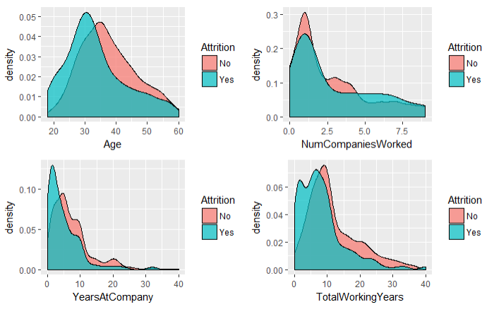
结论:
1.年龄较低的员工的离职率较高,主要集中在30岁以下的员工
2.工作过的企业数量越多越容易离职
3.在公司工作的时间越久,越不容易离职
4.工龄低的员工离职的几率比较大
3.2性别,职位等级,教育背景,部门的分析
# 离职员工的性别分布
g5 <- ggplot(Attr.df, aes(x= Gender,fill = Attrition)) +
  geom_bar(position = "fill") +
  labs(y="Percentage") + scale_y_continuous(labels=percent)

# 离职员工的职位等级分布
g6 <-ggplot(Attr.df, aes(x= JobLevel,fill = Attrition)) +
  geom_bar(position = "fill") + labs(y="Percentage") +
  scale_y_continuous(labels=percent)

# 离职员工的教育背景分布
g7 <- ggplot(Attr.df, aes(x= Education,fill = Attrition)) +
  geom_bar(position = "fill") + labs(y="Percentage") +
  scale_y_continuous(labels=percent)

# 离职员工的部门分布
g8 <- ggplot(Attr.df, aes(x= Department,fill = Attrition)) +
  geom_bar(position = "fill") + labs(y="Percentage") +
  scale_y_continuous(labels=percent) grid.arrange(g5, g6, g7, g8, ncol = 2, nrow = 2)
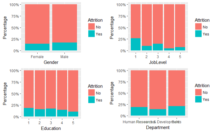
结论:
1.男性的离职率比女性稍高
2.等级越高离职的可能性越小,但是主要集中1级别的职场新人
3.学历和离职率没有太大的关联
4.销售部门相对于其他两个部门离职率较高
3.3 探索涨薪比例,培训次数,每年晋升,员工股权的分析
# 离职员工与涨薪比例的关系
g11 <- ggplot(Attr.df, aes(x = PercentSalaryHike, fill = Attrition)) +
  geom_density(alpha = 0.7)

# 离职员工与培训次数的关系
g12 <- ggplot(Attr.df, aes(x= TrainingTimesLastYear,  group=Attrition)) +
  geom_bar(aes(y = ..prop.., fill = Attrition),
           stat="count", alpha = 0.7,position = "identity",color="black") +
  labs(y="Percentage") + scale_y_continuous(labels=percent)

# 离职员工的与每年晋升的关系
g13 <- ggplot(Attr.df, aes(x = YearsSinceLastPromotion, fill = Attrition)) +
  geom_density(alpha = 0.7)

# 离职员工与股票期权的关系
g14 <- ggplot(Attr.df, aes(x= StockOptionLevel,  group=Attrition)) +
  geom_bar(aes(y = ..prop.., fill = Attrition),
           stat="count", alpha = 0.7,position = "identity",color="black") +
  labs(y="Percentage") + scale_y_continuous(labels=percent)

grid.arrange(g11, g12, g13, g14, ncol = 2)
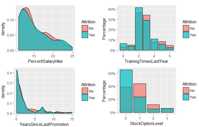
结论:
1.没有涨薪计划的员工流失率较高
2.培训次数和离职率没有太大的影响
3.没有晋升的员工离职率较高
4.没有股权的员工流失率较大
3.4探索工作满意度,同事满意度,环境满意度的分析
# 离职员工与工作满意度的关系
g15 <- ggplot(Attr.df, aes(x= JobSatisfaction,  group=Attrition)) +
  geom_bar(aes(y = ..prop.., fill = Attrition),
           stat="count", alpha = 0.7,position = "identity",color="black") +
  labs(y="Percentage") + scale_y_continuous(labels=percent)

# 离职员工与同事满意度的关系
g16 <- ggplot(Attr.df, aes(x= RelationshipSatisfaction,  group=Attrition)) +
  geom_bar(aes(y = ..prop.., fill = Attrition),
           stat="count", alpha = 0.7,position = "identity",color="black") +
  labs(y="Percentage") + scale_y_continuous(labels=percent)

# 离职员工与工作环境满意度的关系
g17 <- ggplot(Attr.df, aes(x= EnvironmentSatisfaction,  group=Attrition)) +
  geom_bar(aes(y = ..prop.., fill = Attrition),
           stat="count", alpha = 0.7,position = "identity",color="black") +
  labs(y="Percentage") + scale_y_continuous(labels=percent)
grid.arrange(g15, g16,g17, ncol = 3)

结论:满意度越高越不容易离职
3.5探索加班,工作生活的平衡性,是否需要出差,家庭距离之间的关系
# 离职员工和加班之间的关系
g18 <- ggplot(Attr.df, aes(x= OverTime,  group=Attrition)) +
  geom_bar(aes(y = ..prop.., fill = Attrition),
           stat="count", alpha = 0.7,position = "identity",color="black") +
  labs(y="Percentage") + scale_y_continuous(labels=percent)

# 离职员工和工作生活之间的关系
g19 <- ggplot(Attr.df, aes(x= WorkLifeBalance,  group=Attrition)) +
  geom_bar(aes(y = ..prop.., fill = Attrition),
           stat="count", alpha = 0.7,position = "identity",color="black") +
  labs(y="Percentage") + scale_y_continuous(labels=percent)

# 离职员工和出差之间的关系
g20 <- ggplot(Attr.df, aes(x= BusinessTravel,  group=Attrition)) +
  geom_bar(aes(y = ..prop.., fill = Attrition),
           stat="count", alpha = 0.7,position = "identity",color="black") +
  labs(y="Percentage") + scale_y_continuous(labels=percent)

# 离职员工和上班距离之间的关系
g21 <- ggplot(Attr.df,aes(x=DistanceFromHome,fill=Attrition))+
  geom_density(alpha=0.7)

grid.arrange(g18, g19,g20,g21, ncol = 2)
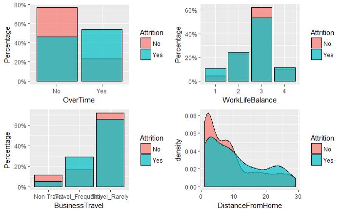
结论:
1.加班越多离职率越高
2.认为工作和生活协调为1的员工工离职率较高
3.经常出差的员工离职率较高
4.距离上班地点越远的员工离职率较高
3.6月薪,职位等级和离职率的关系
# 离职员工和月薪的关系
g9 <- ggplot(Attr.df,aes(x=MonthlyIncome,fill=Attrition))+
  geom_density(alpha=0.7)

# 离职员工与职位等级的关系
g10 <- ggplot(Attr.df, aes(x= JobInvolvement,  group=Attrition)) +
  geom_bar(aes(y = ..prop.., fill = Attrition),
           stat="count", alpha = 0.7,position = "identity",color="black") +
  labs(y="Percentage") + scale_y_continuous(labels=percent)

grid.arrange(g9, g10, ncol = 2)
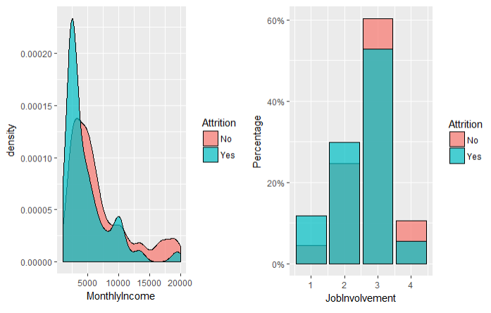
结论:
1.月薪低的员工容易离职
2.职位级别低的离职率较高,但不是很明显
3.6进一步分析月薪和职位级别的关系
ggplot(Attr.df,aes(x=JobInvolvement,y=MonthlyIncome,group=JobInvolvement))+
  geom_boxplot(aes(fill=factor(..x..)),alpha=0.7)+
  theme(legend.position = 'none',plot.title = element_text(hjust = 0.5))+
  facet_grid(~Attrition)+ggtitle('Attrition')

结论:可以明显的得出收入的高低并不是影响员工离职的最主要的因素,如果付出和回报不成正比,会有极大的员工流动
4.建模
4.1决策树
# 去除数据集中没有必要的因子
levels(Attr.df$JobRole) <- c("HC", "HR", "Lab", "Man", "MDir", "RsD", "RsSci", "SlEx", "SlRep")
levels(Attr.df$EducationField) <- c("HR", "LS", "MRK", "MED", "NA", "TD")
Attr.df <- Attr.df[c(-9,-10,-22,-27)]
# 把数据集划分成训练集和测试集
n <- nrow(Attr.df)
rnd <- sample(n,n*0.7)
train <- Attr.df[rnd,]
test <- Attr.df[-rnd,]
# 建模
dtree <- rpart(Attrition~.,data=train)
preds <- predict(dtree,test,type='class')
rocv <- roc(as.numeric(test$Attrition),as.numeric(preds))
rocv$auc
prop.table(table(test$Attrition,preds,dnn = c('Actual','Predicted')),1)
dtreepr <- prune(dtree,cp=0.01666667)
predspr <- predict(dtreepr,test,type='class')
rocvpr <- roc(as.numeric(test$Attrition),as.numeric(predspr))
rocvpr$auc
rpart.plot(dtreepr,type=4,extra=104,tweak = 0.9,fallen.leaves = F,cex = 0.7)
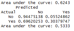
结论:AUC的值0.624比较低,而且灵敏度0.3说明该模型并不能很好的预测离职
4.2随机森林
set.seed(2343)
fit.forest <- randomForest(Attrition~.,data=train)
rfpreds <- predict(fit.forest,test,type='class')
rocrf <- roc(as.numeric(test$Attrition),as.numeric(rfpreds))
rocrf$auc

结论:需要进行优化
4.3GBM
set.seed(3443)
# 定义10折交叉验证用于控制所有的GBM模型训练
ctrl <- trainControl(method = 'cv',number=10,summaryFunction = twoClassSummary,classProbs = T)
gbmfit <- train(Attrition~.,data=train,method='gbm',verbose=F,metric='ROC',trControl=ctrl)
gbmpreds <- predict(gbmfit,test)
rocgbm <- roc(as.numeric(test$Attrition),as.numeric(gbmpreds))
rocgbm$auc

结论:需要进行优化
4.4优化GBM模型
# 设置和之前一样的种子数
ctrl$seeds <- gbmfit$control$seeds

# 加权GBM,设置权重参数,平衡样本
model_weights <- ifelse(train$Attrition == 'No',
                        (1/table(train$Attrition)[1]),
                        (1/table(train$Attrition)[2]))


weightedleft <- train(Attrition ~ .,
                      data=train,
                      method='gbm',
                      verbose=F,
                      weights=model_weights,
                      metric='ROC',
                      trControl=ctrl)

weightedpreds <- predict(weightedleft,test)
rocweight <- roc(as.numeric(test$Attrition),as.numeric(weightedpreds))
rocweight$auc

# 向上采样
ctrl$sampling <- 'up'
set.seed(3433)
upfit <- train(Attrition ~.,
               data = train,
               method = "gbm",
               verbose = FALSE,
               metric = "ROC",
               trControl = ctrl)

uppreds <- predict(upfit, test)
rocup <- roc(as.numeric(test$Attrition), as.numeric(uppreds))
rocup$auc

# 向下采样
ctrl$sampling <- 'down'
set.seed(3433)
downfit <- train(Attrition ~.,
               data = train,
               method = "gbm",
               verbose = FALSE,
               metric = "ROC",
               trControl = ctrl)

downpreds <- predict(downfit, test)
rocdown <- roc(as.numeric(test$Attrition), as.numeric(downpreds))
rocdown$auc

prop.table(table(test$Attrition, weightedpreds, dnn = c("Actual", "Predicted")),1)

结论:选取第二车向上采样的模型,精确度提升到72%,灵敏度提升到62%
5 使用模型来预测离职
5.1查看哪些因素影响员工离职
varImp(upfit)
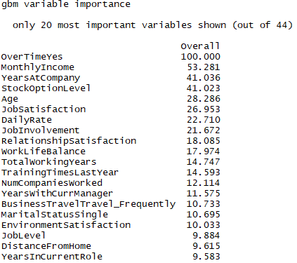
结论:影响员工离职的首要因素:加班,月薪,在公司工作的年限,是否有股权,年龄等因素
5.2预测工作投入高,月薪少的员工的离职率
upfitprobs <- predict(upfit,test,type = 'prob')
test$Prediction <- upfitprobs$Yes
ggplot(test,
       aes(x=MonthlyIncome,y=Prediction,color=factor(JobInvolvement)))+
  geom_point(alpha=0.7)+
  geom_smooth(method = 'lm')+
  facet_wrap(~JobInvolvement)+
  theme(legend.position = 'none')+
  ggtitle('JobInvolvement')+
  theme(plot.title = element_text(hjust = 0.5))
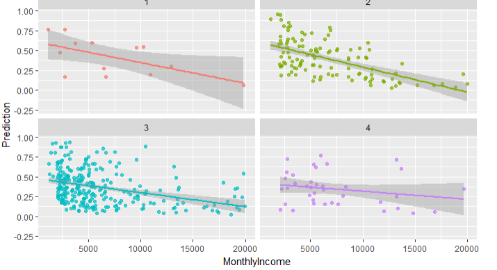
结论:图4表示工作投入高,但是月薪低的员工反而是不容易离职的,可能是因为对企业有归属感或者是企业的其他福利待遇较好
5.3预测那些职位的离职率最高
ggplot(test,aes(x=JobRole,y=Prediction,fill=JobRole))+
  geom_boxplot(alpha=0.5)+
  theme(legend.position = 'none')+
  scale_y_continuous(labels = percent)

结论:销售的离职率相对与其他的离职率较大
总结:
1.员工离职的很大原因是因为加班,或者是付出和回报不成正比导致的
2.在某些生活方面,比如频繁出差,上班路程较远也是员工离职的一个次要原因
3.相比于高薪的吸引力,员工更加认可股权的享有,享有股权分红的员工更不容易离职
4.年龄,在公司的年限和工龄也是影响员工离职的一些重要的指标
5.如果有更多的真实数据集,模型可能会更加准确
github:https://github.com/Mounment/R-Project