matlab中自带的计算距离矩阵的函数有两个pdist和pdist2。前者计算一个向量自身的距离矩阵,后者计算两个向量之间的距离矩阵。基本调用形式如下:
D = pdist(X)
D = pdist2(X,Y)
这两个函数都提供多种距离度量形式,非常方便,还可以调用自己编写的距离函数。
需要注意的是:pdist2返回是n*n的距离矩阵,pdist则返回距离矩阵的下三角串联形式。
下面是具体的介绍:
一、pdist
Pairwise distance between pairs of objects
Syntax
D = pdist(X)
D = pdist(X,distance)
Description
D = pdist(X)
计算 X 中各对行向量的相互距离(X是一个m-by-n的矩阵). 这里 D 要特别注意,D 是一个长为m(m–1)/2的行向量.可以这样理解 D 的生成:首先生成一个 X 的距离方阵,由于该方阵是对称的,且对角线上的元素为0,所以取此方阵的下三角元素,按照Matlab中矩阵的按列存储原则,此下三角各元素的索引排列即为(2,1), (3,1), ..., (m,1), (3,2), ..., (m,2), ..., (m,m–1).可以用命令 squareform(D) 将此行向量转换为原距离方阵.(squareform函数是专门干这事的,其逆变换是也是squareform。)
D = pdist(X,distance) 使用指定的距离.distance可以取下面圆括号中的值,用红色标出!
Metrics
Given an m-by-n data matrix X, which is treated as m (1-by-n) row vectors x1, x2, ..., xm, the various distances between the vector xs and xt are defined as follows:
欧几里德距离Euclidean distance('euclidean')
d 2 s,t =(x s x t )(x s x t ) ′
Notice that the Euclidean distance is a special case of the Minkowski metric, where p = 2.
欧氏距离虽然很有用,但也有明显的缺点。
一:它将样品的不同属性(即各指标或各变量)之间的差别等同看待,这一点有时不能满足实际要求。
二:它没有考虑各变量的数量级(量纲),容易犯大数吃小数的毛病。所以,可以先对原始数据进行规范化处理再进行距离计算。
标准欧几里德距离Standardized Euclidean distance('seuclidean')
d 2 s,t =(x s x t )V 1 (x s x t ) ′
where V is the n-by-n diagonal matrix whose jth diagonal element is S(j)2, where S is the vector of standard deviations.
相比单纯的欧氏距离,标准欧氏距离能够有效的解决上述缺点。注意,这里的V在许多Matlab函数中是可以自己设定的,不一定非得取标准差,可以依据各变量的重要程度设置不同的值,如knnsearch函数中的Scale属性。
马哈拉诺比斯距离Mahalanobis distance('mahalanobis')
d 2 s,t =(x s x t )C 1 (x s x t ) ′
where C is the covariance matrix.
马氏距离是由印度统计学家马哈拉诺比斯(P. C. Mahalanobis)提出的,表示数据的协方差距离。它是一种有效的计算两个未知样本集的相似度的方法。与欧式距离不同的是它考虑到各种特性之间的联系(例如:一条关于身高的信息会带来一条关于体重的信息,因为两者是有关联的)并且是尺度无关的(scale-invariant),即独立于测量尺度。
如果协方差矩阵为单位矩阵,那么马氏距离就简化为欧式距离,如果协方差矩阵为对角阵,则其也可称为正规化的欧氏距离.
马氏优缺点:
1)马氏距离的计算是建立在总体样本的基础上的,因为C是由总样本计算而来,所以马氏距离的计算是不稳定的;
2)在计算马氏距离过程中,要求总体样本数大于样本的维数。
3)协方差矩阵的逆矩阵可能不存在。
曼哈顿距离(城市区块距离)City block metric('cityblock')
d s,t =∑ j=1 n ∣ ∣ x s j x t j ∣ ∣
Notice that the city block distance is a special case of the Minkowski metric, where p=1.
闵可夫斯基距离Minkowski metric('minkowski')
d s,t =∑ j=1 n ∣ ∣ x s j x t j ∣ ∣ p p
Notice that for the special case of p = 1, the Minkowski metric gives the city block metric, for the special case of p = 2, the Minkowski metric gives the Euclidean distance, and for the special case of p = ∞, the Minkowski metric gives the Chebychev distance.
闵可夫斯基距离由于是欧氏距离的推广,所以其缺点与欧氏距离大致相同。
切比雪夫距离Chebychev distance('chebychev')
d s,t =max j ∣ ∣ x s j x t j ∣ ∣
Notice that the Chebychev distance is a special case of the Minkowski metric, where p = ∞.
夹角余弦距离Cosine distance('cosine')
d s,t =1x s x t ′ ∥x s ∥ 2 ∥x t ∥ 2
与Jaccard距离相比,Cosine距离不仅忽略0-0匹配,而且能够处理非二元向量,即考虑到变量值的大小。
相关距离Correlation distance('correlation')
d s,t =1x s x t ′ (x s x s ˉ ˉ ˉ )(x s x s ˉ ˉ ˉ ) ′ √ (x t x t ˉ ˉ ˉ )(x t x t ˉ ˉ ˉ ) ′ √
Correlation距离主要用来度量两个向量的线性相关程度。
汉明距离Hamming distance('hamming')
d s,t =(#(x s j ≠x t j ) n )
两个向量之间的汉明距离的定义为两个向量不同的变量个数所占变量总数的百分比。
杰卡德距离Jaccard distance('jaccard')
d s,t =#[(x s j ≠x t j )∩((x s j ≠0)∪(x t j ≠0))] #[(x s j ≠0)∪(x t j ≠0)]
Jaccard距离常用来处理仅包含非对称的二元(0-1)属性的对象。很显然,Jaccard距离不关心0-0匹配,而Hamming距离关心0-0匹配。
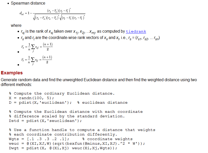
Spearman distance('spearman')
d s,t =1(r s r s ˉ ˉ ˉ )(r t r t ˉ ˉ ˉ ) ′ (r s r s ˉ ˉ ˉ )(r s r s ˉ ˉ ˉ ) ′ √ (r t r t ˉ ˉ ˉ )(r t r t ˉ ˉ ˉ ) ′ √
where
rsj is the rank of xsj taken over x1j, x2j, ...xmj, as computed by tiedrank
rs and rt are the coordinate-wise rank vectors of xs and xt, i.e., rs = (rs1, rs2, ... rsn)
r s ˉ ˉ ˉ =1 n ∑ j r s j =n+1 2
r t ˉ ˉ ˉ =1 n ∑ j r t j =n+1 2
二、pdist2
Pairwise distance between two sets of observations
Syntax
D = pdist2(X,Y)
D = pdist2(X,Y,distance)
D = pdist2(X,Y,'minkowski',P)
D = pdist2(X,Y,'mahalanobis',C)
D = pdist2(X,Y,distance,'Smallest',K)
D = pdist2(X,Y,distance,'Largest',K)
[D,I] = pdist2(X,Y,distance,'Smallest',K)
[D,I] = pdist2(X,Y,distance,'Largest',K)
Description
这里 X 是 mx-by-n 维矩阵,Y 是 my-by-n 维矩阵,生成 mx-by-my 维距离矩阵 D。
[D,I] = pdist2(X,Y,distance,'Smallest',K)
生成 K-by-my 维矩阵 D 和同维矩阵 I,其中D的每列是原距离矩阵中最小的元素,按从小到大排列,I 中对应的列即为其索引号。注意,这里每列各自独立地取 K 个最小值。
例如,令原mx-by-my 维距离矩阵为A,则 K-by-my 维矩阵 D 满足 D(:,j)=A(I(:,j),j).
此外,
MATLAB 距离计算
判别分析时,通常涉及到计算两个样本之间的距离,多元统计学理论中有多种距离计算公式。MATLAB中已有对应函数,可方便直接调用计算。距离函数有:pdist, pdist2, mahal, squareform, mdscale, cmdscale
主要介绍pdist2 ,其它可参考matlab help
D = pdist2(X,Y)
D = pdist2(X,Y,distance)
D = pdist2(X,Y,'minkowski',P)
D = pdist2(X,Y,'mahalanobis',C)
D = pdist2(X,Y,distance,'Smallest',K)
D = pdist2(X,Y,distance,'Largest',K)
[D,I] = pdist2(X,Y,distance,'Smallest',K)
[D,I] = pdist2(X,Y,distance,'Largest',K)
练习:
2种计算方式,一种直接利用pdist计算,另一种按公式(见最后理论)直接计算。
% distance
clc;clear;
x = rand(4,3)
y = rand(1,3)
for i =1:size(x,1)
for j =1:size(y,1)
a = x(i,:); b=y(j,:);
% Euclidean distance
d1(i,j)=sqrt((a-b)*(a-b)');
% Standardized Euclidean distance
V = diag(1./std(x).^2);
d2(i,j)=sqrt((a-b)*V*(a-b)');
% Mahalanobis distance
C = cov(x);
d3(i,j)=sqrt((a-b)*pinv(C)*(a-b)');
% City block metric
d4(i,j)=sum(abs(a-b));
% Minkowski metric
p=3;
d5(i,j)=(sum(abs(a-b).^p))^(1/p);
% Chebychev distance
d6(i,j)=max(abs(a-b));
% Cosine distance
d7(i,j)=1-(a*b')/sqrt(a*a'*b*b');
% Correlation distance
ac = a-mean(a); bc = b-mean(b);
d8(i,j)=1- ac*bc'/(sqrt(sum(ac.^2))*sqrt(sum(bc.^2)));
end
end
md1 = pdist2(x,y,'Euclidean');
md2 = pdist2(x,y,'seuclidean');
md3 = pdist2(x,y,'mahalanobis');
md4 = pdist2(x,y,'cityblock');
md5 = pdist2(x,y,'minkowski',p);
md6 = pdist2(x,y,'chebychev');
md7 = pdist2(x,y,'cosine');
md8 = pdist2(x,y,'correlation');
md9 = pdist2(x,y,'hamming');
md10 = pdist2(x,y,'jaccard');
md11 = pdist2(x,y,'spearman');
D1=[d1,md1],D2=[d2,md2],D3=[d3,md3]
D4=[d4,md4],D5=[d5,md5],D6=[d6,md6]
D7=[d7,md7],D8=[d8,md8]
md9,md10,md11
运行结果如下:
x =
0.5225 0.6382 0.6837
0.3972 0.5454 0.2888
0.8135 0.0440 0.0690
0.6608 0.5943 0.8384
y =
0.5898 0.7848 0.4977
D1 =
0.2462 0.2462
0.3716 0.3716
0.8848 0.8848
0.3967 0.3967
D2 =
0.8355 0.8355
1.5003 1.5003
3.1915 3.1915
1.2483 1.2483
D3 =
439.5074 439.5074
437.5606 437.5606
438.3339 438.3339
437.2702 437.2702
D4 =
0.3999 0.3999
0.6410 0.6410
1.3934 1.3934
0.6021 0.6021
D5 =
0.2147 0.2147
0.3107 0.3107
0.7919 0.7919
0.3603 0.3603
D6 =
0.1860 0.1860
0.2395 0.2395
0.7409 0.7409
0.3406 0.3406
D7 =
0.0253 0.0253
0.0022 0.0022
0.3904 0.3904
0.0531 0.0531
D8 =
1.0731 1.0731
0.0066 0.0066
1.2308 1.2308
1.8954 1.8954
md9 =
1
1
1
1
md10 =
1
1
1
1
md11 =
1.5000
0.0000
1.5000
2.0000
基本理论公式如下: