scikit-learn 是非常优秀的一个有关机器学习的 Python Lib,包含了除深度学习之外的传统机器学习的绝大多数算法,对于了解传统机器学习是一个很不错的平台。每个算法都有相应的例子,既可以对算法有个大概的了解,而且还能熟悉这个工具包的应用,同时也能熟悉 Python 的一些技巧。
Ordinary Least Squares
我们先来看看最常见的线性模型,线性回归是机器学习里很常见的一类问题。
这里我们把向量 称为系数,把 称为截距。
线性回归就是为了解决如下的问题:
sklearn 可以很方便的调用线性模型去做线性回归拟合:
import matplotlib.pyplot as plt
import numpy as np
from sklearn import datasets, linear_model
from sklearn.metrics import mean_squared_error, r2_score

data_set = datasets.load_diabetes()
data_x = data_set.data[:, np.newaxis, 2]

x_train = data_x [:-20]
x_test = data_x[-20:]

y_train = data_set.target[:-20]
y_test = data_set.target[-20:]

regr = linear_model.LinearRegression()
regr.fit(x_train, y_train)
y_pred = regr.predict(x_test)

print('coefficients:
', regr.coef_)
print('mean squared error: %.2f' % mean_squared_error(y_test, y_pred))
print('variance scores: %.2f' % r2_score(y_test, y_pred))

plt.scatter(x_test, y_test, color = 'black')
plt.plot(x_test, y_pred, color = 'blue', linewidth=3)

plt.xticks(())
plt.yticks(())

plt.show()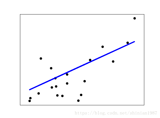
Ridge Regression
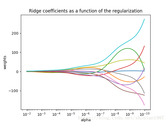
上面介绍的是最常见的一种最小二乘线性拟合,这种线性拟合不带正则惩罚项,对系数没有任何约束,在高维空间中容易造成过拟合,一般来说,最小二乘拟合都会带正则项,比如下面这种:
这种带二范数的正则项,称为 ridge regression,其中 控制系数摆动的幅度, 越大,系数越平滑,意味着系数的方差越小,系数越趋于一种线性关系。下面这个例子给出了 与系数之间的关系:
import matplotlib.pyplot as plt
from sklearn import linear_model
import numpy as np

X = 1. / ( np.arange(1, 11) + np.arange(0, 10)[:, np.newaxis] )

# broadcasting
# a = np.arange(1, 11) + np.arange(0, 10)[:, np.newaxis]

y = np.ones(10)

n_alphas = 100
alphas = np.logspace(-10, -2, n_alphas)

coefs = []

for a in alphas:
    ridge = linear_model.Ridge(alpha=a, fit_intercept=False)
    ridge.fit(X, y)
    coefs.append(ridge.coef_)

ax = plt.gca()

ax.plot(alphas, coefs)
ax.set_xscale('log')
# reverse the axis
ax.set_xlim(ax.get_xlim()[::-1])

plt.xlabel('alpha')
plt.ylabel('weights')
plt.title('Ridge coefficients as a function of the regularization')
plt.axis('title')

plt.show()