机器学习: Tensor Flow +CNN 做笑脸识别

Tensor Flow 是一个采用数据流图（data flow graphs），用于数值计算的开源软件库。节点（Nodes）在图中表示数学操作，图中的线（edges）则表示在节点间相互联系的多维数据数组，即张量（tensor）。

这是谷歌开源的一个强大的做深度学习的软件库，提供了C++ 和 Python 接口，下面给出用Tensor Flow 建立CNN 网络做笑脸识别的一个简单用例。

我们用到的数据库是GENKI4K，这个数据库有4000张图像，首先做人脸检测与剪切，将图像resize到 64×64 的大小，然后用一个 CNN 网络做识别。

网络的基本结构如下：

input -> conv 1 -> pool 1 -> conv 2 -> pool 2 -> conv 3 -> pool 3 -> fc 1 -> out

input -> 64×64
conv 1 -> filter size: 5×5, output: 60×60
pool 1 -> filter size: 2×2, output: 30×30
conv 2 -> filter size: 7×7, output: 24×24
pool 2 -> filter size: 2×2, output: 12×12
conv 3 -> filter size: 5×5, output: 8×8
pool 3 -> filter size: 2×2, output: 4×4
fc 1 -> hidden nodes: 100, output: 1×100
out -> 1×2

import string, os, sys
import numpy as np
import matplotlib.pyplot as plt
import scipy.io
import random
import tensorflow as tf

# set the folder path
dir_name = 'GENKI4K/Feature_Data'

# set the file path
files = os.listdir(dir_name)
for f in files:
    print (dir_name + os.sep + f)

file_path = dir_name + os.sep + files[10]

# get the data
dic_mat = scipy.io.loadmat(file_path)
data_mat = dic_mat['Face_64']
file_path2 = dir_name + os.sep + files[15]

dic_label = scipy.io.loadmat(file_path2)
label_mat = dic_label['Label']
file_path3 = dir_name + os.sep+files[16]

# get the label
label = label_mat.ravel()

label_y = np.zeros((4000, 2))

label_y[:, 0] = label
label_y[:, 1] = 1-label

T_ind=random.sample(range(0, 4000), 4000)


# Parameters
learning_rate = 0.001
batch_size = 40
batch_num=4000/batch_size
train_epoch=100

# Network Parameters
n_input = 4096 # data input (img shape: 64*64)
n_classes = 2 # total classes (smile & non-smile)
dropout = 0.5 # Dropout, probability to keep units

# tf Graph input
x = tf.placeholder(tf.float32, [None, n_input])
y = tf.placeholder(tf.float32, [None, n_classes])
keep_prob = tf.placeholder(tf.float32) #dropout (keep probability)


# Create some wrappers for simplicity
def conv2d(x, W, b, strides=1):
    # Conv2D wrapper, with bias and relu activation
    x = tf.nn.conv2d(x, W, strides=[1, strides, strides, 1], padding='VALID')
    x = tf.nn.bias_add(x, b)
    return tf.nn.relu(x)

def maxpool2d(x, k=2):
    # MaxPool2D wrapper
    return tf.nn.max_pool(x, ksize=[1, k, k, 1], strides=[1, k, k, 1],
                          padding='VALID')

# Create model
def conv_net(x, weights, biases, dropout):
    # Reshape input picture
    x = tf.reshape(x, shape=[-1, 64, 64, 1])

    # Convolution Layer
    conv1 = conv2d(x, weights['wc1'], biases['bc1'])
    # Max Pooling (down-sampling)
    conv1 = maxpool2d(conv1, k=2)

    # Convolution Layer
    conv2 = conv2d(conv1, weights['wc2'], biases['bc2'])
    # Max Pooling (down-sampling)
    conv2 = maxpool2d(conv2, k=2)

    # Convolution Layer
    conv3 = conv2d(conv2, weights['wc3'], biases['bc3'])
    # Max Pooling (down-sampling)
    conv3 = maxpool2d(conv3, k=2)


    # Fully connected layer
    # Reshape conv2 output to fit fully connected layer input
    fc1 = tf.reshape(conv3, [-1, weights['wd1'].get_shape().as_list()[0]])
    fc1 = tf.add(tf.matmul(fc1, weights['wd1']), biases['bd1'])
    fc1 = tf.nn.relu(fc1)

    # Apply Dropout
    # fc1 = tf.nn.dropout(fc1, dropout)

    # Output, class prediction
    out = tf.add(tf.matmul(fc1, weights['out']), biases['out'])

    return out

# Store layers weight & bias
weights = {
    # 5x5 conv, 1 input, 16 outputs
    'wc1': tf.Variable(tf.random_normal([5, 5, 1, 16])),
    # 7x7 conv, 16 inputs, 8 outputs
    'wc2': tf.Variable(tf.random_normal([7, 7, 16, 8])),
    # 5x5 conv, 8 inputs, 16 outputs
    'wc3': tf.Variable(tf.random_normal([5, 5, 8, 16])),
    # fully connected, 7*7*64 inputs, 1024 outputs
    'wd1': tf.Variable(tf.random_normal([4*4*16, 100])),
    # 1024 inputs, 10 outputs (class prediction)
    'out': tf.Variable(tf.random_normal([100, n_classes]))
}

biases = {
    'bc1': tf.Variable(tf.random_normal([16])),
    'bc2': tf.Variable(tf.random_normal([8])),
    'bc3': tf.Variable(tf.random_normal([16])),
    'bd1': tf.Variable(tf.random_normal([100])),
    'out': tf.Variable(tf.random_normal([n_classes]))
}

# Construct model
pred = conv_net(x, weights, biases, keep_prob)


# Define loss and optimizer
cost = tf.reduce_mean(tf.nn.softmax_cross_entropy_with_logits(pred, y))
optimizer = tf.train.AdamOptimizer(learning_rate=learning_rate).minimize(cost)

# Evaluate model
correct_pred = tf.equal(tf.argmax(pred, 1), tf.argmax(y, 1))
accuracy = tf.reduce_mean(tf.cast(correct_pred, tf.float32))

# Initializing the variables
init = tf.initialize_all_variables()

with tf.Session() as sess:
    sess.run(init)
    for epoch in range(0, train_epoch):
        for batch in range (0, batch_num):
            arr_3 = T_ind[batch * batch_size:(batch + 1) * batch_size]
            batch_x = data_mat[arr_3, :]
            batch_y = label_y[arr_3, :]
            # Run optimization op (backprop)
            sess.run(optimizer, feed_dict={x: batch_x, y: batch_y,
                                           keep_prob: dropout})



        # Calculate loss and accuracy
        loss, acc = sess.run([cost, accuracy], feed_dict={x: data_mat,
                                                              y: label_y,
                                                              keep_prob: 1.})

        print("Epoch: " + str(epoch) + ", Loss= " + 
                  "{:.3f}".format(loss) + ", Training Accuracy= " + 
                  "{:.3f}".format(acc))

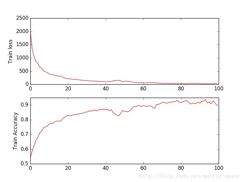
100个训练周期的结果：