[CIKM2019] AutoInt: Automatic Feature Interaction Learning via Self-Attentive Neural Networks

像CTR预估这种任务在推荐系统或者在线广告当中十分常见，但是这个问题也非常具有挑战性，比如所使用的输入特征都是离散并且高维的，有效的预测依赖于高阶组合特征（又称交叉特征）。因此，人们一直在努力寻找稀疏和高维原始特征的低维表示及其有意义的组合。

这篇论文提出了AutoInt来学习高阶特征的交叉表示。并且提出了一个具有残差连接的多头自关注力神经网络，以明确地模拟低维空间中的特征互动。通过多头自关注神经网络的不同层，可以对输入特征的不同顺序组合进行建模，另外还可以提供更强的解释性。整个模型可以以端到端的方式在大规模原始数据上进行有效的拟合。

其他方法的缺点

这篇论文也提到了传统的FM模型的缺点，受到其多项式拟合时间的限制，它只对低阶特征的相互作用建模有效，而对高阶特征的相互作用则不切实际。

再就是兴起的深度模型的缺点，首先，全连接的神经网络在学习特征交叉的相互作用方面被证明是低效的。其次，由于这些模型是以隐含的方式学习特征的相互作用，它们对哪些特征组合是有意义的缺乏良好的解释。

因此，这篇论文正在寻找一种能够明确地对不同顺序的特征组合进行建模的方法，将整个特征表示为低维空间，同时提供良好的模型解释能力。

这篇论文能够处理分类特征和数字特征，具体来说，分类和数字特征首先被嵌入到低维空间中，这就降低了输入特征的维度，同时允许不同类型的特征通过向量运算相互影响。

内容

这篇论文以CTR预估作为问题的背景，首先是一些基本的定义，将用户向量(u)和物品向量(v)进行级联成新的向量(x)，通过这个向量(x)对用户点击物品的概率进行估计。一种最直接最简单的办法就是直接把向量(x)当成输入特征进行逻辑回归。然而，通常来说，向量(x)一般是稀疏的并且高维的，非常容易过拟合。因此，将输入特征在低维空间进行表示是很有必要的。

然后这里定义了p-order Combinatorial Feature，我这里翻译为p阶组合特征。假设我们有输入向量(xin mathbb{R}^n)，那么我们定义p阶组合特征为(g(x_{i_1},x_{i_1},...,x_{i_p}))，其中，(g(cdot))代表非加性函数，可以使叉乘或者点乘等操作。(g(cdot))对多少个特征点进行操作，所得到的结果就是多少阶。这很好理解。

这里目标就有两个，生成有效的高阶特征向量，并且映射到低维空间当中。

AutoInt可以自动学习特征交叉的过程，编码成能够将不同的特征域映射到相同的低维特征空间当中，然后将映射后的特征送入到注意力层当中学习特征交叉，不同的特征交叉的效果通过映射，投影到不同的子空间中的方式由注意力机制进行评价。

如下图所示，是本篇论文AutoInt的模型图。

输入层

我们接着介绍上图的每一层，从下到上首先是输入层

[mathbf{x}=[mathbf{x_1};mathbf{x_2};...;mathbf{x_M}] ]

如果(mathbf{x_i})是种类的话，就使用one-hot向量进行表示，如果(mathbf{x_i})是数值类型的话，我们就使用标量进行表示。

编码层

然后是编码层，由于种类特征是使用one-hot这种稀疏的特征进行表示的，我们对每个种类特征进行了映射编码，

[mathbf{e_i}=mathbf{V_i}mathbf{x_i} ]

那么，(mathbf{V_i})在这里就是编码矩阵。

这里也会有一种情况出现，那就是可能输入的种类特征是multi-hot向量表示的，比如从属多个类别，那么映射的函数发生了一点修改，

[mathbf{e_i}=frac{1}{q}mathbf{V_i}mathbf{x_i} ]

这里的(q)表示了multi-hot特征向量中有多少个值。

为了使得种类特征和数值型特征能够进行交互，那么我们需要将数值型特征也映射到相同的低维空间当中。那么方程可以表示为

[mathbf{e_m}=mathbf{v_m}x_m ]

其中，(x_m)是数值型的特征。那么，所有的编码层工作都介绍完毕。

交互层

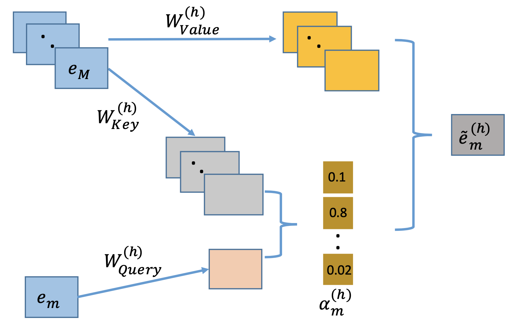
本文使用的是多头自注意力网络，它在对复杂关系进行建模时有着良好的表现。这篇论文用了Key-Value注意力网络来决定哪些特征组合是有意义的。我们以特征(m)举例来说，我们首先定义在明确的注意力头(h)下的特征(m)与特征(k)之间的关系：

[alpha_{mathbf{m,k}}^{(mathbf{h})}=frac{exp(psi^{(h)}(mathbf{e_m,e_k}))}{sum_{l=1}^{M}exp(psi^{(h)}(mathbf{e_m,e_l}))} ]

[psi^{(h)}(mathbf{e_m,e_k})=<mathbf{W_{Query}^{(h)}e_m,W_{Key}^{(h)}e_k}> ]

这里的(psi(cdot))指的是注意力函数，用来表示两个特征的相似性，可以用神经网络表示，或者简单地内积也可以。这篇论文使用了内积的形式。这两个(mathbf{W})是权重矩阵，或者说是转换矩阵，将特征向量投影到新的空间当中。然后我们用所有相关的特征在注意力头(h)下对特征(m)进行更新

[mathbf{widetilde{e}_m^{h}}=sum_{k=1}^{M}alpha_{mathbf{m,k}}^{(mathbf{h})}(mathbf{W_{Value}^{(h)}e_k}) ]

上述特征包含了特征(m)以及相关特征（在注意力头(h)的作用下）的一种组合表示，这样我们就可以得到在不同子空间当中新的离散特征交互的表示方式。

我们把所有注意力头学习的特征进行组合：

[mathbf{widetilde{e}_m}=mathbf{widetilde{e}_m^{(1)}}oplusmathbf{widetilde{e}_m^{(2)}}opluscdotsoplusmathbf{widetilde{e}_m^{(H)}} ]

这里的(oplus)代表的级联操作，(H)表示的注意力头的数量。

为了保持原有的学习到的组合特征，这里就加入了喜闻乐见的残差表示，那么公式发生了进行了进一步变化：

[mathbf{widetilde{e}_m^{RES}}=ReLU(mathbf{widetilde{e}_m}+W_{Res}mathbf{e_m}) ]

这样通过交互层的特征就被完整的表示了出来。这种交互的层可以进行叠加，形成随意阶的组合特征。整个交互层可以通过如下图进行表示。

输出层

交互层的输出是从残差模块里面的原生特征以及经过多头注意力机制的组合特征，为了进行CTR预估，我们简单地将他们进行级联（concatenate）操作，然后进行一次非线性映射进行预测。

[hat y=sigma(mathbf{w^T}(mathbf{e_{1}^{Res}}oplusmathbf{e_{2}^{Res}}opluscdotsoplusmathbf{e_{M}^{Res}})+b) ]

训练

这里的优化目标就是log损失函数：

[Logloss=-frac{1}{N}sum_{j=1}^{N}(y_jlog(hat y_j)+(1-y_j)log(1-hat y_j)) ]

在这里所需要优化的目标就是各种投影方程以及偏置项。

代码

import torch
import torch.nn as nn
import torch.nn.functional as F
from torch.nn.init import xavier_normal_, constant_

from recbole.model.abstract_recommender import ContextRecommender
from recbole.model.layers import MLPLayers

class AutoInt(ContextRecommender):
    """ AutoInt is a novel CTR prediction model based on self-attention mechanism,
    which can automatically learn high-order feature interactions in an explicit fashion.

    """

    def __init__(self, config, dataset):
        super(AutoInt, self).__init__(config, dataset)

        # load parameters info
        self.attention_size = config['attention_size']
        self.dropout_probs = config['dropout_probs']
        self.n_layers = config['n_layers']
        self.num_heads = config['num_heads']
        self.mlp_hidden_size = config['mlp_hidden_size']
        self.has_residual = config['has_residual']

        # define layers and loss
        self.att_embedding = nn.Linear(self.embedding_size, self.attention_size)
        self.embed_output_dim = self.num_feature_field * self.embedding_size
        self.atten_output_dim = self.num_feature_field * self.attention_size
        size_list = [self.embed_output_dim] + self.mlp_hidden_size
        self.mlp_layers = MLPLayers(size_list, dropout=self.dropout_probs[1])
        # multi-head self-attention network
        self.self_attns = nn.ModuleList([
            nn.MultiheadAttention(self.attention_size, self.num_heads, dropout=self.dropout_probs[0])
            for _ in range(self.n_layers)
        ])
        self.attn_fc = torch.nn.Linear(self.atten_output_dim, 1)
        self.deep_predict_layer = nn.Linear(self.mlp_hidden_size[-1], 1)
        if self.has_residual:
            self.v_res_res_embedding = torch.nn.Linear(self.embedding_size, self.attention_size)

        self.dropout_layer = nn.Dropout(p=self.dropout_probs[2])
        self.sigmoid = nn.Sigmoid()
        self.loss = nn.BCELoss()

        # parameters initialization
        self.apply(self._init_weights)

    def _init_weights(self, module):
        if isinstance(module, nn.Embedding):
            xavier_normal_(module.weight.data)
        elif isinstance(module, nn.Linear):
            xavier_normal_(module.weight.data)
            if module.bias is not None:
                constant_(module.bias.data, 0)

    def autoint_layer(self, infeature):
        """ Get the attention-based feature interaction score

        Args:
            infeature (torch.FloatTensor): input feature embedding tensor. shape of[batch_size,field_size,embed_dim].

        Returns:
            torch.FloatTensor: Result of score. shape of [batch_size,1] .
        """

        att_infeature = self.att_embedding(infeature)
        cross_term = att_infeature.transpose(0, 1)
        for self_attn in self.self_attns:
            cross_term, _ = self_attn(cross_term, cross_term, cross_term)
        cross_term = cross_term.transpose(0, 1)
        # Residual connection
        if self.has_residual:
            v_res = self.v_res_embedding(infeature)
            cross_term += v_res
        # Interacting layer
        cross_term = F.relu(cross_term).contiguous().view(-1, self.atten_output_dim)
        batch_size = infeature.shape[0]
        att_output = self.attn_fc(cross_term) + self.deep_predict_layer(self.mlp_layers(infeature.view(batch_size, -1)))
        return att_output

    def forward(self, interaction):
        autoint_all_embeddings = self.concat_embed_input_fields(interaction)  # [batch_size, num_field, embed_dim]
        output = self.first_order_linear(interaction) + self.autoint_layer(autoint_all_embeddings)
        return self.sigmoid(output.squeeze(1))

    def calculate_loss(self, interaction):
        label = interaction[self.LABEL]
        output = self.forward(interaction)
        return self.loss(output, label)

    def predict(self, interaction):
        return self.forward(interaction)