python 求职 Top10 城市，来看看是否有你所在的城市

前言

从智联招聘爬取相关信息后，我们关心的是如何对内容进行分析，获取用用的信息。

本次以上篇文章“5分钟掌握智联招聘网站爬取并保存到MongoDB数据库”中爬取的数据为基础，分析关键词为“python”的爬取数据的情况，获取包括全国python招聘数量Top10的城市列表以及其他相关信息。

一、主要分析步骤

• 数据读取
• 数据整理
• 对职位数量在全国主要城市的分布情况进行分析
• 对全国范围内的职位月薪情况进行分析
• 对该职位招聘岗位要求描述进行词云图分析，获取频率最高的关键字
• 选取两个城市，分别分析月薪分布情况以及招聘要求的词云图分析

二、具体分析过程

import pymongo
import pandas as pd
import matplotlib.pyplot as plt
import numpy as np
% matplotlib inline
plt.style.use('ggplot')

# 解决matplotlib显示中文问题
plt.rcParams['font.sans-serif'] = ['SimHei']  # 指定默认字体
plt.rcParams['axes.unicode_minus'] = False  # 解决保存图像是负号'-'显示为方块的问题

1 读取数据

client = pymongo.MongoClient('localhost')
db = client['zhilian']
table = db['python']

columns = ['zwmc',
           'gsmc',
           'zwyx',
           'gbsj',
           'gzdd',
           'fkl',
           'brief',
           'zw_link',
           '_id',
           'save_date']

# url_set =  set([records['zw_link'] for records in table.find()])
# print(url_set)

df = pd.DataFrame([records for records in table.find()], columns=columns)

# columns_update = ['职位名称',
#                   '公司名称',
#                   '职位月薪',
#                   '公布时间',
#                   '工作地点',
#                   '反馈率',
#                   '招聘简介',
#                   '网页链接',
#                   '_id',
#                   '信息保存日期']
# df.columns = columns_update
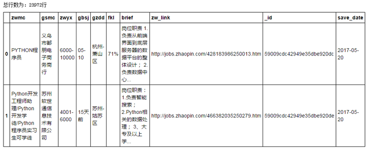
print('总行数为：{}行'.format(df.shape[0]))
df.head(2)

欢迎加入我的QQ群`923414804`与我一起学习，群里有我学习过程中整理的大量学习资料。加群即可免费获取

结果如图1所示：

2 数据整理

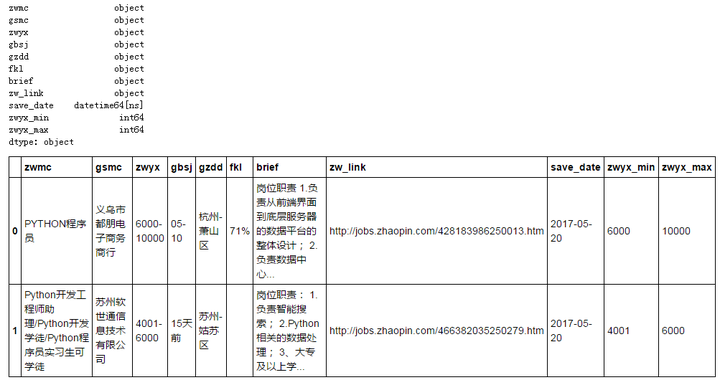
2.1 将str格式的日期变为 datatime

df['save_date'] = pd.to_datetime(df['save_date'])
print(df['save_date'].dtype)
# df['save_date']

datetime64[ns]

2.2 筛选月薪格式为“XXXX-XXXX”的信息

df_clean = df[['zwmc',
           'gsmc',
           'zwyx',
           'gbsj',
           'gzdd',
           'fkl',
           'brief',
           'zw_link',
           'save_date']]

# 对月薪的数据进行筛选，选取格式为“XXXX-XXXX”的信息，方面后续分析
df_clean = df_clean[df_clean['zwyx'].str.contains('d+-d+', regex=True)]
print('总行数为：{}行'.format(df_clean.shape[0]))
# df_clean.head()

总行数为：22605行

2.3 分割月薪字段，分别获取月薪的下限值和上限值

# Pandas DataFrame, how do i split a column into two

# Append column to pandas dataframe

# df_temp.loc[: ,'zwyx_min'],df_temp.loc[: , 'zwyx_max'] = df_temp.loc[: , 'zwyx'].str.split('-',1).str #会有警告
s_min, s_max = df_clean.loc[: , 'zwyx'].str.split('-',1).str
df_min = pd.DataFrame(s_min)
df_min.columns = ['zwyx_min']
df_max = pd.DataFrame(s_max)
df_max.columns = ['zwyx_max']

df_clean_concat = pd.concat([df_clean, df_min, df_max], axis=1)
# df_clean['zwyx_min'].astype(int)
df_clean_concat['zwyx_min'] = pd.to_numeric(df_clean_concat['zwyx_min'])
df_clean_concat['zwyx_max'] = pd.to_numeric(df_clean_concat['zwyx_max'])
# print(df_clean['zwyx_min'].dtype)
print(df_clean_concat.dtypes)
df_clean_concat.head(2)

运行结果如图2所示：

• 将数据信息按职位月薪进行排序

df_clean_concat.sort_values('zwyx_min',inplace=True)
# df_clean_concat.tail()

• 判断爬取的数据是否有重复值

# 判断爬取的数据是否有重复值
print(df_clean_concat[df_clean_concat.duplicated('zw_link')==True])

Empty DataFrame
Columns: [zwmc, gsmc, zwyx, gbsj, gzdd, fkl, brief, zw_link, save_date, zwyx_min, zwyx_max]
Index: []

• 从上述结果可看出，数据是没有重复的。

3 对全国范围内的职位进行分析

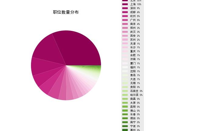
3.1 主要城市的招聘职位数量分布情况

# from IPython.core.display import display, HTML
ADDRESS = [ '北京', '上海', '广州', '深圳',
           '天津', '武汉', '西安', '成都', '大连',
           '长春', '沈阳', '南京', '济南', '青岛',
           '杭州', '苏州', '无锡', '宁波', '重庆',
           '郑州', '长沙', '福州', '厦门', '哈尔滨',
           '石家庄', '合肥', '惠州', '太原', '昆明',
           '烟台', '佛山', '南昌', '贵阳', '南宁']
df_city = df_clean_concat.copy()

# 由于工作地点的写上，比如北京，包含许多地址为北京-朝阳区等
# 可以用替换的方式进行整理，这里用pandas的replace()方法
for city in ADDRESS:
    df_city['gzdd'] = df_city['gzdd'].replace([(city+'.*')],[city],regex=True)

# 针对全国主要城市进行分析
df_city_main = df_city[df_city['gzdd'].isin(ADDRESS)]

df_city_main_count = df_city_main.groupby('gzdd')['zwmc','gsmc'].count()
df_city_main_count['gsmc'] = df_city_main_count['gsmc']/(df_city_main_count['gsmc'].sum())
df_city_main_count.columns = ['number', 'percentage']

# 按职位数量进行排序
df_city_main_count.sort_values(by='number', ascending=False, inplace=True)

# 添加辅助列，标注城市和百分比，方面在后续绘图时使用
df_city_main_count['label']=df_city_main_count.index+ ' '+  ((df_city_main_count['percentage']*100).round()).astype('int').astype('str')+'%'
print(type(df_city_main_count))

# 职位数量最多的Top10城市的列表
print(df_city_main_count.head(10))

<class 'pandas.core.frame.DataFrame'>
      number  percentage   label
gzdd                            
北京      6936    0.315948  北京 32%
上海      3213    0.146358  上海 15%
深圳      1908    0.086913   深圳 9%
成都      1290    0.058762   成都 6%
杭州      1174    0.053478   杭州 5%
广州      1167    0.053159   广州 5%
南京       826    0.037626   南京 4%
郑州       741    0.033754   郑州 3%
武汉       552    0.025145   武汉 3%
西安       473    0.021546   西安 2%

• 对结果进行绘图：

from  matplotlib import cm

label = df_city_main_count['label']
sizes = df_city_main_count['number']

# 设置绘图区域大小
fig, axes = plt.subplots(figsize=(10,6),ncols=2)
ax1, ax2 = axes.ravel()

colors = cm.PiYG(np.arange(len(sizes))/len(sizes)) # colormaps: Paired, autumn, rainbow, gray,spring,Darks

# 由于城市数量太多，饼图中不显示labels和百分比
patches, texts = ax1.pie(sizes,labels=None, shadow=False, startangle=0, colors=colors)

ax1.axis('equal')  

ax1.set_title('职位数量分布', loc='center')

# ax2 只显示图例（legend）
ax2.axis('off')
ax2.legend(patches, label, loc='center left', fontsize=9)

plt.savefig('job_distribute.jpg')
plt.show()

运行结果如下述饼图所示：

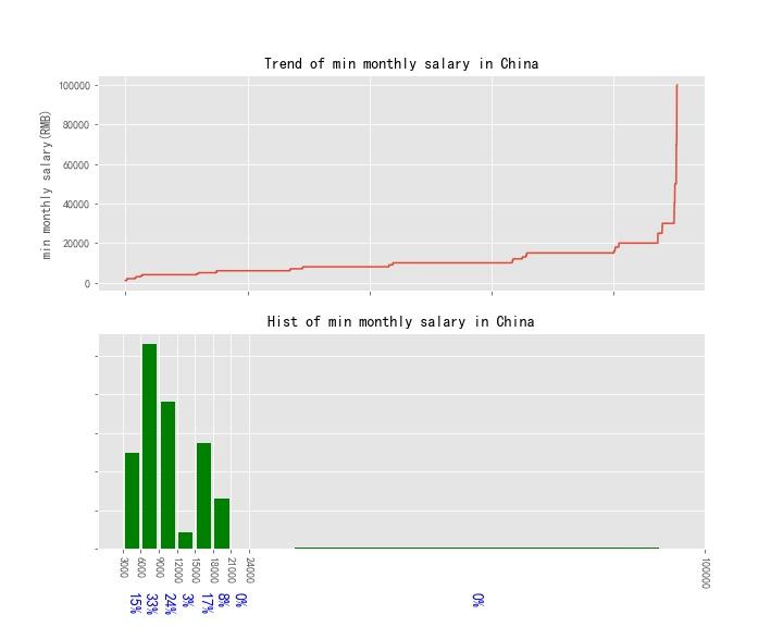
3.2 月薪分布情况（全国）

from matplotlib.ticker import FormatStrFormatter

fig, (ax1, ax2) = plt.subplots(figsize=(10,8), nrows=2)

x_pos = list(range(df_clean_concat.shape[0]))
y1 = df_clean_concat['zwyx_min']

ax1.plot(x_pos, y1)
ax1.set_title('Trend of min monthly salary in China', size=14)
ax1.set_xticklabels('')
ax1.set_ylabel('min monthly salary(RMB)')

bins = [3000,6000, 9000, 12000, 15000, 18000, 21000, 24000, 100000]
counts, bins, patches = ax2.hist(y1, bins, normed=1, histtype='bar', facecolor='g', rwidth=0.8)
ax2.set_title('Hist of min monthly salary in China', size=14)
ax2.set_yticklabels('')
# ax2.set_xlabel('min monthly salary(RMB)')

# Matplotlib - label each bin
ax2.set_xticks(bins) #将bins设置为xticks
ax2.set_xticklabels(bins, rotation=-90) # 设置为xticklabels的方向

# Label the raw counts and the percentages below the x-axis...
bin_centers = 0.5 * np.diff(bins) + bins[:-1]
for count, x in zip(counts, bin_centers):
#     # Label the raw counts
#     ax2.annotate(str(count), xy=(x, 0), xycoords=('data', 'axes fraction'),
#         xytext=(0, -70), textcoords='offset points', va='top', ha='center', rotation=-90)

    # Label the percentages
    percent = '%0.0f%%' % (100 * float(count) / counts.sum())
    ax2.annotate(percent, xy=(x, 0), xycoords=('data', 'axes fraction'),
        xytext=(0, -40), textcoords='offset points', va='top', ha='center', rotation=-90, color='b', size=14)

fig.savefig('salary_quanguo_min.jpg')

运行结果如下述图所示：

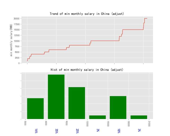
不考虑部分极值后，分析月薪分布情况

df_zwyx_adjust = df_clean_concat[df_clean_concat['zwyx_min']<=20000]

fig, (ax1, ax2) = plt.subplots(figsize=(10,8), nrows=2)

x_pos = list(range(df_zwyx_adjust.shape[0]))
y1 = df_zwyx_adjust['zwyx_min']

ax1.plot(x_pos, y1)
ax1.set_title('Trend of min monthly salary in China (adjust)', size=14)
ax1.set_xticklabels('')
ax1.set_ylabel('min monthly salary(RMB)')

bins = [3000,6000, 9000, 12000, 15000, 18000, 21000]
counts, bins, patches = ax2.hist(y1, bins, normed=1, histtype='bar', facecolor='g', rwidth=0.8)
ax2.set_title('Hist of min monthly salary in China (adjust)', size=14)
ax2.set_yticklabels('')
# ax2.set_xlabel('min monthly salary(RMB)')

# Matplotlib - label each bin
ax2.set_xticks(bins) #将bins设置为xticks
ax2.set_xticklabels(bins, rotation=-90) # 设置为xticklabels的方向

# Label the raw counts and the percentages below the x-axis...
bin_centers = 0.5 * np.diff(bins) + bins[:-1]
for count, x in zip(counts, bin_centers):
#     # Label the raw counts
#     ax2.annotate(str(count), xy=(x, 0), xycoords=('data', 'axes fraction'),
#         xytext=(0, -70), textcoords='offset points', va='top', ha='center', rotation=-90)

    # Label the percentages
    percent = '%0.0f%%' % (100 * float(count) / counts.sum())
    ax2.annotate(percent, xy=(x, 0), xycoords=('data', 'axes fraction'),
        xytext=(0, -40), textcoords='offset points', va='top', ha='center', rotation=-90, color='b', size=14)

fig.savefig('salary_quanguo_min_adjust.jpg')

运行结果如下述图所示：

3.3 相关技能要求

brief_list = list(df_clean_concat['brief'])
brief_str = ''.join(brief_list)
print(type(brief_str))
# print(brief_str)
# with open('brief_quanguo.txt', 'w', encoding='utf-8') as f:
#     f.write(brief_str)

<class 'str'>

对获取到的职位招聘要求进行词云图分析，代码如下：

# -*- coding: utf-8 -*-
"""
Created on Wed May 17 2017

@author: lemon
"""

import jieba
from wordcloud import WordCloud, ImageColorGenerator
import matplotlib.pyplot as plt
import os
import PIL.Image as Image
import numpy as np

with open('brief_quanguo.txt', 'rb') as f: # 读取文件内容
    text = f.read()
    f.close()

# 首先使用 jieba 中文分词工具进行分词
wordlist = jieba.cut(text, cut_all=False)      
# cut_all, True为全模式，False为精确模式

wordlist_space_split = ' '.join(wordlist)

d = os.path.dirname(__file__)
alice_coloring = np.array(Image.open(os.path.join(d,'colors.png')))
my_wordcloud = WordCloud(background_color='#F0F8FF', max_words=100, mask=alice_coloring,
                         max_font_size=300, random_state=42).generate(wordlist_space_split)

image_colors = ImageColorGenerator(alice_coloring)

plt.show(my_wordcloud.recolor(color_func=image_colors))
plt.imshow(my_wordcloud)            # 以图片的形式显示词云
plt.axis('off')                     # 关闭坐标轴
plt.show()

my_wordcloud.to_file(os.path.join(d, 'brief_quanguo_colors_cloud.png'))

得到结果如下：

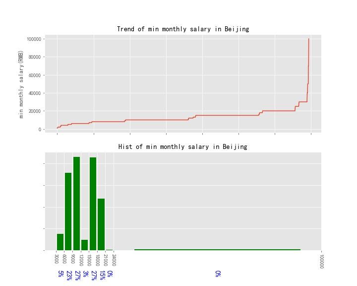
4 北京

4.1 月薪分布情况

df_beijing = df_clean_concat[df_clean_concat['gzdd'].str.contains('北京.*', regex=True)]
df_beijing.to_excel('zhilian_kw_python_bj.xlsx')
print('总行数为：{}行'.format(df_beijing.shape[0]))
# df_beijing.head()

总行数为：6936行

参考全国分析时的代码，月薪分布情况图如下：

4.2 相关技能要求

brief_list_bj = list(df_beijing['brief'])
brief_str_bj = ''.join(brief_list_bj)
print(type(brief_str_bj))
# print(brief_str_bj)
# with open('brief_beijing.txt', 'w', encoding='utf-8') as f:
#     f.write(brief_str_bj)

<class 'str'>

词云图如下：

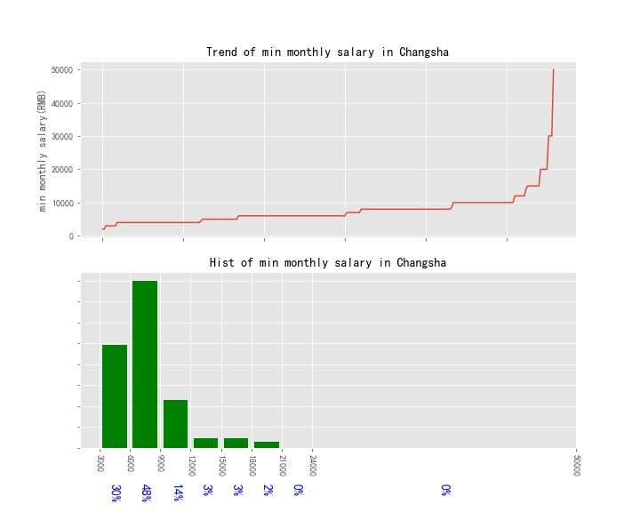
5 长沙

5.1 月薪分布情况

df_changsha = df_clean_concat[df_clean_concat['gzdd'].str.contains('长沙.*', regex=True)]
# df_changsha = pd.DataFrame(df_changsha, ignore_index=True)
df_changsha.to_excel('zhilian_kw_python_cs.xlsx')
print('总行数为：{}行'.format(df_changsha.shape[0]))
# df_changsha.tail()

总行数为：280行

参考全国分析时的代码，月薪分布情况图如下：

5.2 相关技能要求

brief_list_cs = list(df_changsha['brief'])
brief_str_cs = ''.join(brief_list_cs)
print(type(brief_str_cs))
# print(brief_str_cs)
# with open('brief_changsha.txt', 'w', encoding='utf-8') as f:
#     f.write(brief_str_cs)

<class 'str'>

词云图如下：