在本章主要内容:
- NumPy基础知识
- 加载iris数据集
- 查看iris数据集
- 用pandas查看iris数据集
- 用NumPy和matplotlib绘图
- 最小机器学习配方 - SVM分类
- 介绍交叉验证
- 以上汇总
- 机器学习概述 - 分类与回归
简介
本章我们将学习如何使用scikit-learn进行预测。 机器学习强调衡量预测能力,并用scikit-learn进行准确和快速的预测。我们将检查iris数据集,该数据集由三种iris的测量结果组成:Iris Setosa,Iris Versicolor和Iris Virginica。
为了衡量预测,我们将:
- 保存一些数据以进行测试
- 仅使用训练数据构建模型
- 测量测试集的预测能力
解决问题的方法
- 类别(Classification):
- 非文本,比如Iris
- 回归
- 聚类
- 降维
-
技术支持 (可以加qq群:887934385)
NumPy基础
数据科学经常处理结构化的数据表。scikit-learn库需要二维NumPy数组。 在本节中,您将学习
- NumPy的shape和dimension
 1   In [1]: import numpy as np
 2
 3     In [2]: np.arange(10)
 4     Out[2]: array([0, 1, 2, 3, 4, 5, 6, 7, 8, 9])
 5
 6     In [3]: array_1 = np.arange(10)
 7
 8     In [4]: array_1.shape
 9     Out[4]: (10,)
10
11     In [5]: array_1.ndim
12     Out[5]: 1
13
14     In [6]: array_1.reshape((5,2))
15     Out[6]:
16     array([[0, 1],
17            [2, 3],
18            [4, 5],
19            [6, 7],
20            [8, 9]])
21
22     In [7]: array_1 = array_1.reshape((5,2))
23
24     In [8]: array_1.ndim
25     Out[8]: 2
- NumPy广播(broadcasting)
 1  In [9]: array_1 + 1
 2     Out[9]:
 3     array([[ 1,  2],
 4            [ 3,  4],
 5            [ 5,  6],
 6            [ 7,  8],
 7            [ 9, 10]])
 8
 9     In [10]: array_2 = np.arange(10)
10
11     In [11]: array_2 * array_2
12     Out[11]: array([ 0,  1,  4,  9, 16, 25, 36, 49, 64, 81])
13
14     In [12]: array_2 = array_2 ** 2 #Note that this is equivalent to array_2 *
15
16     In [13]: array_2
17     Out[13]: array([ 0,  1,  4,  9, 16, 25, 36, 49, 64, 81])
18
19     In [14]: array_2 = array_2.reshape((5,2))
20
21     In [15]: array_2
22     Out[15]:
23     array([[ 0,  1],
24            [ 4,  9],
25            [16, 25],
26            [36, 49],
27            [64, 81]])
28
29     In [16]: array_1 = array_1 + 1
30
31     In [17]: array_1
32     Out[17]:
33     array([[ 1,  2],
34            [ 3,  4],
35            [ 5,  6],
36            [ 7,  8],
37            [ 9, 10]])
38
39     In [18]: array_1 + array_2
40     Out[18]:
41     array([[ 1,  3],
42            [ 7, 13],
43            [21, 31],
44            [43, 57],
45            [73, 91]])
- 初始化NumPy数组和dtypes
 1   In [19]: np.zeros((5,2))
 2     Out[19]:
 3     array([[0., 0.],
 4            [0., 0.],
 5            [0., 0.],
 6            [0., 0.],
 7            [0., 0.]])
 8
 9     In [20]: np.ones((5,2), dtype = np.int)
10     Out[20]:
11     array([[1, 1],
12            [1, 1],
13            [1, 1],
14            [1, 1],
15            [1, 1]])
16
17     In [21]: np.empty((5,2), dtype = np.float)
18     Out[21]:
19     array([[0.00000000e+000, 0.00000000e+000],
20
21
22            [6.90082649e-310, 6.90082647e-310],
23            [6.90072710e-310, 6.90072711e-310],
24            [6.90083466e-310, 0.00000000e+000],
25            [6.90083921e-310, 1.90979621e-310]])
- 索引
 1  In [22]: array_1[0,0] #Finds value in first row and first column.
 2     Out[22]: 1
 3
 4     In [23]: array_1[0,:] # View the first row
 5     Out[23]: array([1, 2])
 6
 7     In [24]: array_1[:,0] # view the first column
 8     Out[24]: array([1, 3, 5, 7, 9])
 9
10     In [25]: array_1[2:5, :]
11     Out[25]:
12     array([[ 5,  6],
13            [ 7,  8],
14            [ 9, 10]])
15
16     In [26]: array_1
17     Out[26]:
18     array([[ 1,  2],
19            [ 3,  4],
20            [ 5,  6],
21            [ 7,  8],
22            [ 9, 10]])
23
24     In [27]: array_1[2:5,0]
25     Out[27]: array([5, 7, 9])
- 布尔数组
 1     In [28]: array_1 > 5
 2     Out[28]:
 3     array([[False, False],
 4            [False, False],
 5            [False,  True],
 6            [ True,  True],
 7            [ True,  True]])
 8
 9     In [29]: array_1[array_1 > 5]
10     Out[29]: array([ 6,  7,  8,  9, 10])
- 算术运算
 1 In [30]: array_1.sum()
 2     Out[30]: 55
 3
 4     In [31]: array_1.sum(axis = 1) # Find all the sums by row:
 5     Out[31]: array([ 3,  7, 11, 15, 19])
 6
 7     In [32]: array_1.sum(axis = 0) # Find all the sums by column
 8     Out[32]: array([25, 30])
 9
10     In [33]: array_1.mean(axis = 0)
11     Out[33]: array([5., 6.])
- NaN值
 1  # Scikit-learn不接受np.nan
 2     In [34]: array_3 = np.array([np.nan, 0, 1, 2, np.nan])
 3
 4     In [35]: np.isnan(array_3)
 5     Out[35]: array([ True, False, False, False,  True])
 6
 7     In [36]: array_3[~np.isnan(array_3)]
 8     Out[36]: array([0., 1., 2.])
 9
10     In [37]: array_3[np.isnan(array_3)] = 0
11
12     In [38]: array_3
13     Out[38]: array([0., 0., 1., 2., 0.])
Scikit-learn只接受实数的二维NumPy数组,没有缺失的np.nan值。从经验来看,最好将np.nan改为某个值丢弃。 就我个人而言,我喜欢跟踪布尔模板并保持数据的形状大致相同,因为这会导致更少的编码错误和更多的编码灵活性。
加载数据
  1 In [1]: import numpy as np
  2
  3 In [2]: import pandas as pd
  4
  5 In [3]: import matplotlib.pyplot as plt
  6
  7 In [4]: from sklearn import datasets
  8
  9 In [5]: iris = datasets.load_iris()
 10
 11 In [6]: iris.data
 12 Out[6]:
 13 array([[5.1, 3.5, 1.4, 0.2],
 14        [4.9, 3. , 1.4, 0.2],
 15        [4.7, 3.2, 1.3, 0.2],
 16        [4.6, 3.1, 1.5, 0.2],
 17        [5. , 3.6, 1.4, 0.2],
 18        [5.4, 3.9, 1.7, 0.4],
 19        [4.6, 3.4, 1.4, 0.3],
 20        [5. , 3.4, 1.5, 0.2],
 21        [4.4, 2.9, 1.4, 0.2],
 22        [4.9, 3.1, 1.5, 0.1],
 23        [5.4, 3.7, 1.5, 0.2],
 24        [4.8, 3.4, 1.6, 0.2],
 25        [4.8, 3. , 1.4, 0.1],
 26        [4.3, 3. , 1.1, 0.1],
 27        [5.8, 4. , 1.2, 0.2],
 28        [5.7, 4.4, 1.5, 0.4],
 29        [5.4, 3.9, 1.3, 0.4],
 30        [5.1, 3.5, 1.4, 0.3],
 31        [5.7, 3.8, 1.7, 0.3],
 32        [5.1, 3.8, 1.5, 0.3],
 33        [5.4, 3.4, 1.7, 0.2],
 34        [5.1, 3.7, 1.5, 0.4],
 35        [4.6, 3.6, 1. , 0.2],
 36        [5.1, 3.3, 1.7, 0.5],
 37        [4.8, 3.4, 1.9, 0.2],
 38        [5. , 3. , 1.6, 0.2],
 39        [5. , 3.4, 1.6, 0.4],
 40        [5.2, 3.5, 1.5, 0.2],
 41        [5.2, 3.4, 1.4, 0.2],
 42        [4.7, 3.2, 1.6, 0.2],
 43        [4.8, 3.1, 1.6, 0.2],
 44        [5.4, 3.4, 1.5, 0.4],
 45        [5.2, 4.1, 1.5, 0.1],
 46        [5.5, 4.2, 1.4, 0.2],
 47        [4.9, 3.1, 1.5, 0.1],
 48        [5. , 3.2, 1.2, 0.2],
 49        [5.5, 3.5, 1.3, 0.2],
 50        [4.9, 3.1, 1.5, 0.1],
 51        [4.4, 3. , 1.3, 0.2],
 52        [5.1, 3.4, 1.5, 0.2],
 53        [5. , 3.5, 1.3, 0.3],
 54        [4.5, 2.3, 1.3, 0.3],
 55        [4.4, 3.2, 1.3, 0.2],
 56        [5. , 3.5, 1.6, 0.6],
 57        [5.1, 3.8, 1.9, 0.4],
 58        [4.8, 3. , 1.4, 0.3],
 59        [5.1, 3.8, 1.6, 0.2],
 60        [4.6, 3.2, 1.4, 0.2],
 61        [5.3, 3.7, 1.5, 0.2],
 62        [5. , 3.3, 1.4, 0.2],
 63        [7. , 3.2, 4.7, 1.4],
 64        [6.4, 3.2, 4.5, 1.5],
 65        [6.9, 3.1, 4.9, 1.5],
 66        [5.5, 2.3, 4. , 1.3],
 67        [6.5, 2.8, 4.6, 1.5],
 68        [5.7, 2.8, 4.5, 1.3],
 69        [6.3, 3.3, 4.7, 1.6],
 70        [4.9, 2.4, 3.3, 1. ],
 71        [6.6, 2.9, 4.6, 1.3],
 72        [5.2, 2.7, 3.9, 1.4],
 73        [5. , 2. , 3.5, 1. ],
 74        [5.9, 3. , 4.2, 1.5],
 75        [6. , 2.2, 4. , 1. ],
 76        [6.1, 2.9, 4.7, 1.4],
 77        [5.6, 2.9, 3.6, 1.3],
 78        [6.7, 3.1, 4.4, 1.4],
 79        [5.6, 3. , 4.5, 1.5],
 80        [5.8, 2.7, 4.1, 1. ],
 81        [6.2, 2.2, 4.5, 1.5],
 82        [5.6, 2.5, 3.9, 1.1],
 83        [5.9, 3.2, 4.8, 1.8],
 84        [6.1, 2.8, 4. , 1.3],
 85        [6.3, 2.5, 4.9, 1.5],
 86        [6.1, 2.8, 4.7, 1.2],
 87        [6.4, 2.9, 4.3, 1.3],
 88        [6.6, 3. , 4.4, 1.4],
 89        [6.8, 2.8, 4.8, 1.4],
 90        [6.7, 3. , 5. , 1.7],
 91        [6. , 2.9, 4.5, 1.5],
 92        [5.7, 2.6, 3.5, 1. ],
 93        [5.5, 2.4, 3.8, 1.1],
 94        [5.5, 2.4, 3.7, 1. ],
 95        [5.8, 2.7, 3.9, 1.2],
 96        [6. , 2.7, 5.1, 1.6],
 97        [5.4, 3. , 4.5, 1.5],
 98        [6. , 3.4, 4.5, 1.6],
 99        [6.7, 3.1, 4.7, 1.5],
100        [6.3, 2.3, 4.4, 1.3],
101        [5.6, 3. , 4.1, 1.3],
102        [5.5, 2.5, 4. , 1.3],
103        [5.5, 2.6, 4.4, 1.2],
104        [6.1, 3. , 4.6, 1.4],
105        [5.8, 2.6, 4. , 1.2],
106        [5. , 2.3, 3.3, 1. ],
107        [5.6, 2.7, 4.2, 1.3],
108        [5.7, 3. , 4.2, 1.2],
109        [5.7, 2.9, 4.2, 1.3],
110        [6.2, 2.9, 4.3, 1.3],
111        [5.1, 2.5, 3. , 1.1],
112        [5.7, 2.8, 4.1, 1.3],
113        [6.3, 3.3, 6. , 2.5],
114        [5.8, 2.7, 5.1, 1.9],
115        [7.1, 3. , 5.9, 2.1],
116        [6.3, 2.9, 5.6, 1.8],
117        [6.5, 3. , 5.8, 2.2],
118        [7.6, 3. , 6.6, 2.1],
119        [4.9, 2.5, 4.5, 1.7],
120        [7.3, 2.9, 6.3, 1.8],
121        [6.7, 2.5, 5.8, 1.8],
122        [7.2, 3.6, 6.1, 2.5],
123        [6.5, 3.2, 5.1, 2. ],
124        [6.4, 2.7, 5.3, 1.9],
125        [6.8, 3. , 5.5, 2.1],
126        [5.7, 2.5, 5. , 2. ],
127        [5.8, 2.8, 5.1, 2.4],
128        [6.4, 3.2, 5.3, 2.3],
129        [6.5, 3. , 5.5, 1.8],
130        [7.7, 3.8, 6.7, 2.2],
131        [7.7, 2.6, 6.9, 2.3],
132        [6. , 2.2, 5. , 1.5],
133        [6.9, 3.2, 5.7, 2.3],
134        [5.6, 2.8, 4.9, 2. ],
135        [7.7, 2.8, 6.7, 2. ],
136        [6.3, 2.7, 4.9, 1.8],
137        [6.7, 3.3, 5.7, 2.1],
138        [7.2, 3.2, 6. , 1.8],
139        [6.2, 2.8, 4.8, 1.8],
140        [6.1, 3. , 4.9, 1.8],
141        [6.4, 2.8, 5.6, 2.1],
142        [7.2, 3. , 5.8, 1.6],
143        [7.4, 2.8, 6.1, 1.9],
144        [7.9, 3.8, 6.4, 2. ],
145        [6.4, 2.8, 5.6, 2.2],
146        [6.3, 2.8, 5.1, 1.5],
147        [6.1, 2.6, 5.6, 1.4],
148        [7.7, 3. , 6.1, 2.3],
149        [6.3, 3.4, 5.6, 2.4],
150        [6.4, 3.1, 5.5, 1.8],
151        [6. , 3. , 4.8, 1.8],
152        [6.9, 3.1, 5.4, 2.1],
153        [6.7, 3.1, 5.6, 2.4],
154        [6.9, 3.1, 5.1, 2.3],
155        [5.8, 2.7, 5.1, 1.9],
156        [6.8, 3.2, 5.9, 2.3],
157        [6.7, 3.3, 5.7, 2.5],
158        [6.7, 3. , 5.2, 2.3],
159        [6.3, 2.5, 5. , 1.9],
160        [6.5, 3. , 5.2, 2. ],
161        [6.2, 3.4, 5.4, 2.3],
162        [5.9, 3. , 5.1, 1.8]])
163
164 In [7]: iris.data.shape
165 Out[7]: (150, 4)
166
167 In [8]: iris.data[0]
168 Out[8]: array([5.1, 3.5, 1.4, 0.2])
169
170 In [9]: iris.feature_names
171 Out[9]:
172 ['sepal length (cm)',
173  'sepal width (cm)',
174  'petal length (cm)',
175  'petal width (cm)']
176
177 In [10]: iris.target
178 Out[10]:
179 array([0, 0, 0, 0, 0, 0, 0, 0, 0, 0, 0, 0, 0, 0, 0, 0, 0, 0, 0, 0, 0, 0,
180        0, 0, 0, 0, 0, 0, 0, 0, 0, 0, 0, 0, 0, 0, 0, 0, 0, 0, 0, 0, 0, 0,
181        0, 0, 0, 0, 0, 0, 1, 1, 1, 1, 1, 1, 1, 1, 1, 1, 1, 1, 1, 1, 1, 1,
182        1, 1, 1, 1, 1, 1, 1, 1, 1, 1, 1, 1, 1, 1, 1, 1, 1, 1, 1, 1, 1, 1,
183        1, 1, 1, 1, 1, 1, 1, 1, 1, 1, 1, 1, 2, 2, 2, 2, 2, 2, 2, 2, 2, 2,
184        2, 2, 2, 2, 2, 2, 2, 2, 2, 2, 2, 2, 2, 2, 2, 2, 2, 2, 2, 2, 2, 2,
185        2, 2, 2, 2, 2, 2, 2, 2, 2, 2, 2, 2, 2, 2, 2, 2, 2, 2])
186
187 In [11]: iris.target.shape
188 Out[11]: (150,)
189
190 In [12]: iris.target_names
191 Out[12]: array(['setosa', 'versicolor', 'virginica'], dtype='<U10')
- 用pandas查看数据
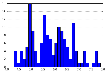
 1 import numpy as np    #Load the numpy library for fast array computations
 2 import pandas as pd   #Load the pandas data-analysis library
 3 import matplotlib.pyplot as plt   #Load the pyplot visualization library
 4
 5 %matplotlib inline
 6
 7 from sklearn import datasets
 8 iris = datasets.load_iris()
 9
10 iris_df = pd.DataFrame(iris.data, columns = iris.feature_names)
11
12 iris_df['sepal length (cm)'].hist(bins=30)
```
!python
for class_number in np.unique(iris.target): plt.figure(1) iris_df['sepal length (cm)'].iloc[np.where(iris.target == class_number)[0]].hist(bins=30)

```
#!python
np.where(iris.target == class_number)[0]
执行结果
1 array([100, 101, 102, 103, 104, 105, 106, 107, 108, 109, 110, 111, 112,
2        113, 114, 115, 116, 117, 118, 119, 120, 121, 122, 123, 124, 125,
3        126, 127, 128, 129, 130, 131, 132, 133, 134, 135, 136, 137, 138,
4        139, 140, 141, 142, 143, 144, 145, 146, 147, 148, 149], dtype=int64)
matplotlib和NumPy作图
 1 import numpy as np
 2 import matplotlib.pyplot as plt
 3 %matplotlib inline
 4
 5 plt.plot(np.arange(10), np.arange(10))
 6
 7 plt.plot(np.arange(10), np.exp(np.arange(10)))
 8
 9
10 # 两张图片放在一起
11 plt.figure()
12 plt.subplot(121)
13 plt.plot(np.arange(10), np.exp(np.arange(10)))
14 plt.subplot(122)
15 plt.scatter(np.arange(10), np.exp(np.arange(10)))
16
17
18
19 plt.figure()
20 plt.subplot(211)
21 plt.plot(np.arange(10), np.exp(np.arange(10)))
22 plt.subplot(212)
23 plt.scatter(np.arange(10), np.exp(np.arange(10)))
24
25 plt.figure()
26 plt.subplot(221)
27 plt.plot(np.arange(10), np.exp(np.arange(10)))
28 plt.subplot(222)
29 plt.scatter(np.arange(10), np.exp(np.arange(10)))
30 plt.subplot(223)
31 plt.scatter(np.arange(10), np.exp(np.arange(10)))
32 plt.subplot(224)
33 plt.scatter(np.arange(10), np.exp(np.arange(10)))
34
35 from sklearn.datasets import load_iris
36
37 iris = load_iris()
38 data = iris.data
39 target = iris.target
40
41 # Resize the figure for better viewing
42 plt.figure(figsize=(12,5))
43
44 # First subplot
45 plt.subplot(121)
46
47 # Visualize the first two columns of data:
48 plt.scatter(data[:,0], data[:,1], c=target)
49
50 # Second subplot
51 plt.subplot(122)
52
53 # Visualize the last two columns of data:
54 plt.scatter(data[:,2], data[:,3], c=target)
1 2 3 4 5 6 7 8 9 10 11 12 13 14 15 16 17 18 19 20 21 22 23 24 25 26 27 28 29 30 31 32 33 34 35 36 37 38 39 40 41 42 43 44 45 46 47 48 49 50 51 52 53 54 |
import numpy as np
import matplotlib.pyplot as plt
%matplotlib inline

plt.plot(np.arange(10), np.arange(10))

plt.plot(np.arange(10), np.exp(np.arange(10)))


# 两张图片放在一起
plt.figure()
plt.subplot(121)
plt.plot(np.arange(10), np.exp(np.arange(10)))
plt.subplot(122)
plt.scatter(np.arange(10), np.exp(np.arange(10)))


plt.figure()
plt.subplot(211)
plt.plot(np.arange(10), np.exp(np.arange(10)))
plt.subplot(212)
plt.scatter(np.arange(10), np.exp(np.arange(10)))

plt.figure()
plt.subplot(221)
plt.plot(np.arange(10), np.exp(np.arange(10)))
plt.subplot(222)
plt.scatter(np.arange(10), np.exp(np.arange(10)))
plt.subplot(223)
plt.scatter(np.arange(10), np.exp(np.arange |