二.线性神经网络

　　自适应线性元件20世纪50年代末由Widrow和Hoff提出，主要用于线性逼近一个函数式而进行模式联想以及信号滤波、预测、模型识别和控制等。

　　线性神经网络和感知器的区别是，感知器只能输出两种可能的值，而线性神经网络的输出可以取任意值。线性神经网络采用Widrow-Hoff学习规则，即LMS（Least Mean Square）算法来调整网络的权值和偏置。线性神经网络在结构上与感知器非常相似，只是神经元激活函数不同。在模型训练时把原来的sign函数改成了pureline函数(y=x)

　　只能解决线性可分的问题。

　　与感知器类似，神经元传输函数不同。

线性神经网络结构

 

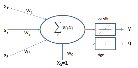
两个激活函数，当训练时用线性purelin函数，训练完成后，输出时用到sign函数　(>0, <0)

假设输入是一个N维向量（公式1）,从输入到神经元的权值为wi，则输出为公式2.

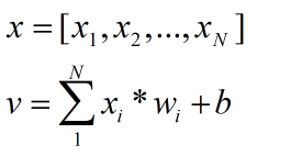
若传递函数采用线性函数purelin，则输入与输出为一个简单的比例关系，x(n),w(n),y,q写成矩阵的形式，公式如下、

若网络中包含多个神经元节点，则可以形成多个输出，这种可以以两种间接的方式解决线性不可分问题

• 用多个线性函数对区域进行划分，然后对各个神经元的输出做逻辑运算
• 或者对神经元添加非线性输入，引入非线性成分。

LMS 最小均方规则

LMS 学习规则可以看作是δ学习规则的一个特殊情况

LMS算法只能训练单层网络，，但是单层网络理论上讲不会比单层网络差。
该学习规则与神经元采用的转移函数无关，因而不需要对转移函数求导，不仅学习速度较快，而且具有较高的精度，权值可以初始化为任意值，通过权值调整使得神经元实际输出与期望输出之间的平方差最小:

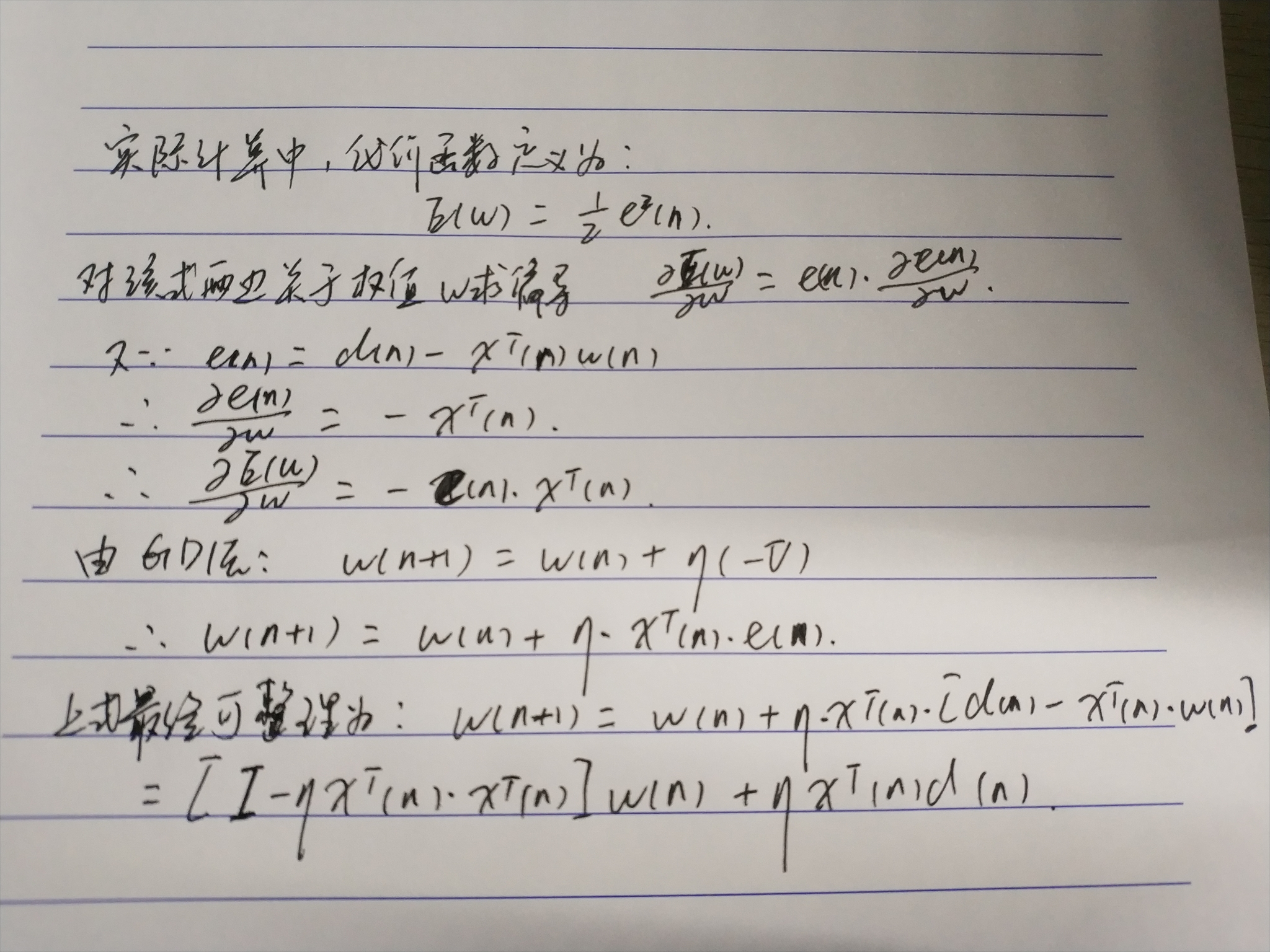
定义某次迭代时的信号为　　e(n)=d(n)-x^T(n)w(n)

n为迭代次数，d表示期望输出，采用均方误差作为评价指标。

Q是输入训练样本的个数。线性神经网络学习的目标是找到适当的w，使得均方差mse最小。mse对w求偏导，令偏导等于0求得mse极值，因为mse 必为正，二次函数凹向上，求得的极值必为极小值。

　　　实际运算中，为了解决权值w维数过高，给计算带来困难，往往调节权值，使mse从空间中的某一点开始，沿着斜面向下滑行，最终达到最小值。滑行的方向使该店最陡下降的方向，即负梯度方向。

　　　实际计算中，代价函数常定义为

　　　　　　　　　　　　　　　　　　　

Delta学习规则

1986年，认知心理学家McClelland和Rumelhart 在神经网络训练中引入该规则，也成为连续感知器学习规则
该学习规则是一种利用梯度下降法的一般性的学习规则

代价函数(损失函数) (Cost Function, Lost Function)

误差E是权向量Wj的函数，欲使误差E最小，Wj应与误差的负梯度成正比

 

梯度即是导数，对误差（代价／损失）函数求导，

 该学习规则可以推广到多层前馈网络中，权值可以初始化为任意值。

梯度下降法的问题

• 学习率难以选取，太大会产生振荡，太小收敛缓慢
• 容易陷入局部最优解
• 第一个问题解决方法，开始的学习率可以设的较大，后面逐渐调小学习率

LMS算法步骤

(1)定义变量和参数。

　　x(n)=N+1维输入向量=[+1,x1(n),x2(n),...,xN(n)]T

　　w(n)=N+1维权值向量=[b(n),w1(n),w2(n),...,wN(n)]T

　　b(n)=偏置

　　y(n)=实际输出

　　d(n)=期望输出

　　η(n)=学习率参数，是一个比1小的正常数

(2)初始化。n=0,将权值向量w设置为随机值或全零值,n=0。

(3)输入样本，计算实际输出和误差，根据给定的期望输出d(n)，计算得:e(n)=d(n)-xT(n)*w(n)

(4)更加所算的的结果调整权值向量（由上图所给公式）

(5)判断算法是否收敛，若满足收敛条件，则算法结束，否则继续

收敛条件：当权值向量w已经能正确实现分类时，算法就收敛了，此时网络误差为零。收敛条件通常可以是：

　　　　误差小于某个预先设定的较小的值ε。即

　　　　　　　　　　　　　　　　　　|e(n)|<ε

　　　　两次迭代之间的权值变化已经很小，即

　　　　　　　　　　　　　　　　　　|w(n+1)-w(n)|<ε

　　　　设定最大迭代次数M，当迭代了M次就停止迭代。

LMS算法中学习率的选择

LMS算法中，学习率的选择十分重要，直接影响了神经网络的性能和收敛性。

　1996年Hayjin证明，只要学习率η满足   LMS算法就是按方差收敛的。

　　　　　　其中，λmax是输入向量x（n）组成的自相关矩阵R的最大特征值。往往使用R的迹（trace）来代替。矩阵的迹是矩阵主对角线元素之和。

　　　　　　可改写成  0<η<2/向量均方值之和。

　　  学习率逐渐下降：

　　　　学习初期，用比较大的学习率保证收敛速度，随着迭代次数增加，减小学习率保证精度，确保收敛。

学习率逐渐下降如何设计：多种方式，自己可以思考思考

线性神经网络与感知器的对比

LMS算法运用梯度下降法用于训练线性神经网络，这个思想后来发展成为反向传播算法用于训练多层神经网络。

两者的传输函数不一样导致感知器只能用于分类，而线性神经网络还可以用于拟合或者逼近

LMS算法的分类边界往往处于两种模式的中间，容错能力强，感知器算法则在刚好能正确分类的地方就停下了，容错能力差。

Python实现LMS算法

#! /usr/bin/env python
# -*- coding:utf-8 -*-
import numpy as np
import pandas as pd


def sgn(x):     # the sgn function
    if x >= 0:
        return 1
    else:
        return -1


class LinearNeuralNetwork(object):
    """
    This is the Perception of the Neural Newtork.
    I implement the algorithm by myself.
    """
    def __init__(self, input_data, input_label, learning_rate=0.05, iter_times=5000):
        """

        :param input_data: is the np.array type and size is [m, n] which m is number of data, n is the length of a input
        :param input_label: is the np.array type and size is [1, m] which m is number of data
        :param learning_rate:
        :param iter_times:
        """
        self.datas = np.ones((input_data.shape[0], input_data.shape[1] + 1))
        self.datas[:, 1:] = input_data
        self.label = input_label
        self.weights = (np.random.random(size=self.datas.shape[1]) - 0.5) * 2    # make the weights in [-1, 1]
        self.learning_rate = learning_rate
        self.iter_times = iter_times
        for i in range(self.iter_times):
            for j in range(self.datas.shape[0]):
                e = self.label[j] - np.dot(self.datas[j], self.weights.T)
                new_w = self.weights + self.learning_rate * e * self.datas[j]
                self.weights = new_w
            if sum(abs(self.label - np.dot(self.datas, self.weights))) <= 0.001:    # if |y(n) - d(n)| <=0.001, break
                print("The perception is work well!")
                break
        print("The real data output:", self.label)
        print("LMS of y  output is :", np.array([x for x in np.dot(self.datas, self.weights.T)]))
        print("LMS of q  output is :", np.array([sgn(x) for x in np.dot(self.datas, self.weights.T)]))

运用实现的LMS算法处理一些数据

#! /usr/bin/env python
# -*- coding:utf-8 -*-
import numpy as np
import pandas as pd


def sgn(x):     # the sgn function
    if x >= 0:
        return 1
    else:
        return -1


class LinearNeuralNetwork(object):
    """
    This is the Perception of the Neural Newtork.
    I implement the algorithm by myself.
    """
    def __init__(self, input_data, input_label, learning_rate=0.05, iter_times=5000):
        """

        :param input_data: is the np.array type and size is [m, n] which m is number of data, n is the length of a input
        :param input_label: is the np.array type and size is [1, m] which m is number of data
        :param learning_rate:
        :param iter_times:
        """
        self.datas = np.ones((input_data.shape[0], input_data.shape[1] + 1))
        self.datas[:, 1:] = input_data
        self.label = input_label
        self.weights = (np.random.random(size=self.datas.shape[1]) - 0.5) * 2    # make the weights in [-1, 1]
        self.learning_rate = learning_rate
        self.iter_times = iter_times
        for i in range(self.iter_times):
            for j in range(self.datas.shape[0]):
                e = self.label[j] - np.dot(self.datas[j], self.weights.T)
                new_w = self.weights + self.learning_rate * e * self.datas[j]
                self.weights = new_w
            if sum(abs(self.label - np.dot(self.datas, self.weights))) <= 0.001:    # if |y(n) - d(n)| <=0.001, break
                print("The perception is work well!")
                break
        print("The real data output:", self.label)
        print("LMS of y  output is :", np.array([x for x in np.dot(self.datas, self.weights.T)]))
        print("LMS of q  output is :", np.array([sgn(x) for x in np.dot(self.datas, self.weights.T)]))


def main():
    X = np.array([[1, 3, 3],
                  [1, 4, 3],
                  [1, 1, 1]])

    Y = np.array([1, 1, -1])
    LinearNeuralNetwork(X, Y)


if __name__ == '__main__':
    main()