介绍
以下介绍和算法引用自选择性搜索(selective search)。
一、目标检测 VS 目标识别
目标识别(objec recognition)是指明一幅输入图像中包含那类目标。其输入为一幅图像,输出是该图像中的目标属于哪个类别(class probability)。而目标检测(object detection)除了要告诉输入图像中包含了哪类目前外,还要框出该目标的具体位置(bounding boxes)。
在目标检测时,为了定位到目标的具体位置,通常会把图像分成许多子块(sub-regions / patches),然后把子块作为输入,送到目标识别的模型中。分子块的最直接方法叫滑动窗口法(sliding window approach)。滑动窗口的方法就是按照子块的大小在整幅图像上穷举所有子图像块。这种方法产生的数据量想想都头大。和滑动窗口法相对的是另外一类基于区域(region proposal)的方法。selective search就是其中之一!
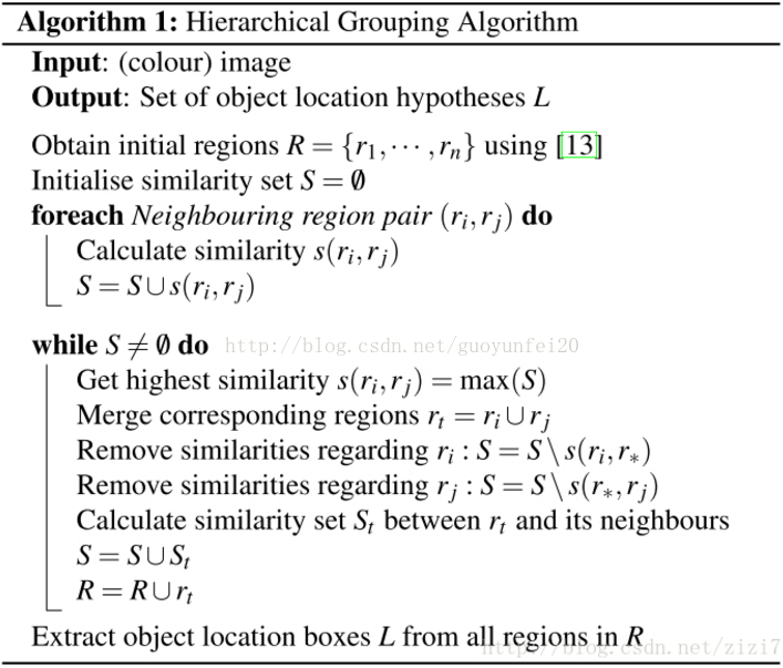
二、selective search算法流程
step0:生成区域集R,具体参见论文《Efficient Graph-Based Image Segmentation》
step1:计算区域集R里每个相邻区域的相似度S={s1,s2,…}
step2:找出相似度最高的两个区域,将其合并为新集,添加进R
step3:从S中移除所有与step2中有关的子集
step4:计算新集与所有子集的相似度
step5:跳至step2,直至S为空三、相似度计算
论文考虑了颜色、纹理、尺寸和空间交叠这4个参数。
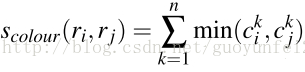
3.1、颜色相似度(color similarity)
将色彩空间转为HSV,每个通道下以bins=25计算直方图,这样每个区域的颜色直方图有25*3=75个区间。 对直方图除以区域尺寸做归一化后使用下式计算相似度:
3.2、纹理相似度(texture similarity)
论文采用方差为1的高斯分布在8个方向做梯度统计,然后将统计结果(尺寸与区域大小一致)以bins=10计算直方图。直方图区间数为8*3*10=240(使用RGB色彩空间)。
其中,
是直方图中第
个bin的值。
3.3、尺寸相似度(size similarity)
保证合并操作的尺度较为均匀,避免一个大区域陆续“吃掉”其他小区域。
例:设有区域a-b-c-d-e-f-g-h。较好的合并方式是:ab-cd-ef-gh -> abcd-efgh -> abcdefgh。 不好的合并方法是:ab-c-d-e-f-g-h ->abcd-e-f-g-h ->abcdef-gh -> abcdefgh。
3.4、交叠相似度(shape compatibility measure)
3.5、最终的相似度


实现
使用了前面几篇提到的一些算法,运行速度慢
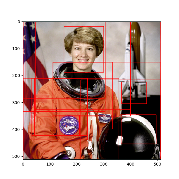
# -*- coding: utf-8 -*-
from __future__ import division
from skimage.color import rgb2hsv
from skimage.data import astronaut
import numpy
from _felzenszwalb_cy import _felzenszwalb_cython
import matplotlib.patches as mpatches
import matplotlib.pyplot as plt
import math

# "Selective Search for Object Recognition" by J.R.R. Uijlings et al.
#
#  - Modified version with LBP extractor for texture vectorization


def _sim_colour(r1, r2):
    """
        calculate the sum of histogram intersection of colour
    """
    return sum([min(a, b) for a, b in zip(r1["hist_c"], r2["hist_c"])])


def _sim_texture(r1, r2):
    """
        calculate the sum of histogram intersection of texture
    """
    return sum([min(a, b) for a, b in zip(r1["hist_t"], r2["hist_t"])])


def _sim_size(r1, r2, imsize):
    """
        calculate the size similarity over the image
    """
    return 1.0 - (r1["size"] + r2["size"]) / imsize


def _sim_fill(r1, r2, imsize):
    """
        calculate the fill similarity over the image
    """
    bbsize = (
        (max(r1["max_x"], r2["max_x"]) - min(r1["min_x"], r2["min_x"]))
        * (max(r1["max_y"], r2["max_y"]) - min(r1["min_y"], r2["min_y"]))
    )
    return 1.0 - (bbsize - r1["size"] - r2["size"]) / imsize


def _calc_sim(r1, r2, imsize):
    return (_sim_colour(r1, r2) + _sim_texture(r1, r2)
            + _sim_size(r1, r2, imsize) + _sim_fill(r1, r2, imsize))


def histogram(a, bins=10, range=None):
    """
    Compute the histogram of a set of data.

    """
    import numpy as numpy
    from numpy.core import linspace
    from numpy.core.numeric import (arange, asarray)
    # 转成一维数组
    a = asarray(a)
    a = a.ravel()
    mn, mx = [mi + 0.0 for mi in range]
    ntype = numpy.dtype(numpy.intp)
    n = numpy.zeros(bins, ntype)
    # 预计算直方图缩放因子
    norm = bins / (mx - mn)

    # 均分,计算边缘以进行潜在的校正
    bin_edges = linspace(mn, mx, bins + 1, endpoint=True)

    # 分块对于大数组可以降低运行内存,同时提高速度
    BLOCK = 65536
    for i in arange(0, len(a), BLOCK):
        tmp_a = a[i:i + BLOCK]
        tmp_a_data = tmp_a.astype(float)
        # 减去Range下限,乘以缩放因子,向下取整
        tmp_a = tmp_a_data - mn
        tmp_a *= norm
        indices = tmp_a.astype(numpy.intp)
        # 对indices标签分别计数,标签等于bins减一
        indices[indices == bins] -= 1
        n += numpy.bincount(indices, weights=None,
                             minlength=bins).astype(ntype)

    return n, bin_edges


def _calc_colour_hist(img):
    """
        calculate colour histogram for each region

        the size of output histogram will be BINS * COLOUR_CHANNELS(3)

        number of bins is 25 as same as [uijlings_ijcv2013_draft.pdf]

        extract HSV
    """

    BINS = 25
    hist = numpy.array([])

    for colour_channel in (0, 1, 2):

        # extracting one colour channel
        c = img[:, colour_channel]

        # calculate histogram for each colour and join to the result
        hist = numpy.concatenate(
        [hist] + [histogram(c, BINS, (0.0, 255.0))[0]])

    # L1 normalize
    hist = hist / len(img)

    return hist

def circular_LBP(src, n_points, radius):
    height = src.shape[0]
    width = src.shape[1]
    dst = src.copy()
    src.astype(dtype=numpy.float32)
    dst.astype(dtype=numpy.float32)

    neighbours = numpy.zeros((1, n_points), dtype=numpy.uint8)
    lbp_value = numpy.zeros((1, n_points), dtype=numpy.uint8)
    for x in range(radius, width - radius - 1):
        for y in range(radius, height - radius - 1):
            lbp = 0.
            # 先计算共n_points个点对应的像素值,使用双线性插值法
            for n in range(n_points):
                theta = float(2 * numpy.pi * n) / n_points
                x_n = x + radius * numpy.cos(theta)
                y_n = y - radius * numpy.sin(theta)

                # 向下取整
                x1 = int(math.floor(x_n))
                y1 = int(math.floor(y_n))
                # 向上取整
                x2 = int(math.ceil(x_n))
                y2 = int(math.ceil(y_n))

                # 将坐标映射到0-1之间
                tx = numpy.abs(x - x1)
                ty = numpy.abs(y - y1)

                # 根据0-1之间的x,y的权重计算公式计算权重
                w1 = (1 - tx) * (1 - ty)
                w2 = tx * (1 - ty)
                w3 = (1 - tx) * ty
                w4 = tx * ty

                # 根据双线性插值公式计算第k个采样点的灰度值
                neighbour = src[y1, x1] * w1 + src[y2, x1] * w2 + src[y1, x2] * w3 + src[y2, x2] * w4

                neighbours[0, n] = neighbour

            center = src[y, x]

            for n in range(n_points):
                if neighbours[0, n] > center:
                    lbp_value[0, n] = 1
                else:
                    lbp_value[0, n] = 0

            for n in range(n_points):
                lbp += lbp_value[0, n] * 2**n

            # 转换到0-255的灰度空间,比如n_points=16位时结果会超出这个范围,对该结果归一化
            dst[y, x] = int(lbp / (2**n_points-1) * 255)

    return dst

def _calc_texture_gradient(img):
    """
        calculate texture gradient for entire image

        The original SelectiveSearch algorithm proposed Gaussian derivative
        for 8 orientations, but we use LBP instead.

        output will be [height(*)][width(*)]
    """
    ret = numpy.zeros((img.shape[0], img.shape[1], img.shape[2]))

    for colour_channel in (0, 1, 2):
        ret[:, :, colour_channel] = circular_LBP(
            img[:, :, colour_channel], 8, 1)

    return ret


def _calc_texture_hist(img):
    """
        calculate texture histogram for each region

        calculate the histogram of gradient for each colours
        the size of output histogram will be
            BINS * ORIENTATIONS * COLOUR_CHANNELS(3)
    """
    BINS = 10

    hist = numpy.array([])

    for colour_channel in (0, 1, 2):

        # mask by the colour channel
        fd = img[:, colour_channel]

        # calculate histogram for each orientation and concatenate them all
        # and join to the result
        hist = numpy.concatenate(
            [hist] + [numpy.histogram(fd, BINS, (0.0, 1.0))[0]])

    # L1 Normalize
    hist = hist / len(img)

    return hist


def _merge_regions(r1, r2):
    new_size = r1["size"] + r2["size"]
    rt = {
        "min_x": min(r1["min_x"], r2["min_x"]),
        "min_y": min(r1["min_y"], r2["min_y"]),
        "max_x": max(r1["max_x"], r2["max_x"]),
        "max_y": max(r1["max_y"], r2["max_y"]),
        "size": new_size,
        "hist_c": (
            r1["hist_c"] * r1["size"] + r2["hist_c"] * r2["size"]) / new_size,
        "hist_t": (
            r1["hist_t"] * r1["size"] + r2["hist_t"] * r2["size"]) / new_size,
        "labels": r1["labels"] + r2["labels"]
    }
    return rt


def selective_search(
        im_orig, scale=1.0, sigma=0.8, min_size=50):

    assert im_orig.shape[2] == 3, "3ch image is expected"

    # 加载图像,使用felzenszwalb算法获取候选区域,区域标签存储到数据的第四维

    im_mask = _felzenszwalb_cython(
        im_orig, scale=scale, sigma=sigma,
        min_size=min_size, kernel=9)
    img = numpy.append(
        im_orig, numpy.zeros(im_orig.shape[:2])[:, :, numpy.newaxis], axis=2)
    img[:, :, 3] = im_mask

    if img is None:
        return None, {}

    imsize = img.shape[0] * img.shape[1]

    R = {}
    hsv = rgb2hsv(img[:, :, :3])
    # 第一步: 存储像素位置
    for y, i in enumerate(img):
        for x, (r, g, b, l) in enumerate(i):
            # 新区域
            if l not in R:
                R[l] = {
                    "min_x": 0xffff, "min_y": 0xffff,
                    "max_x": 0, "max_y": 0, "labels": [l]}

            # bounding box
            if R[l]["min_x"] > x:
                R[l]["min_x"] = x
            if R[l]["min_y"] > y:
                R[l]["min_y"] = y
            if R[l]["max_x"] < x:
                R[l]["max_x"] = x
            if R[l]["max_y"] < y:
                R[l]["max_y"] = y

    # 第二步: 计算LBP纹理特征
    tex_grad = _calc_texture_gradient(img)

    # 第三步: 计算每个区域的颜色直方图
    for k, v in list(R.items()):
        masked_pixels = hsv[:, :, :][img[:, :, 3] == k]
        R[k]["size"] = len(masked_pixels)  # /4
        R[k]["hist_c"] = _calc_colour_hist(masked_pixels)
        R[k]["hist_t"] = _calc_texture_hist(tex_grad[:, :][img[:, :, 3] == k])

    # 提取邻域信息
    def intersect(a, b):
        if (a["min_x"] < b["min_x"] < a["max_x"]
                and a["min_y"] < b["min_y"] < a["max_y"]) or (
            a["min_x"] < b["max_x"] < a["max_x"]
                and a["min_y"] < b["max_y"] < a["max_y"]) or (
            a["min_x"] < b["min_x"] < a["max_x"]
                and a["min_y"] < b["max_y"] < a["max_y"]) or (
            a["min_x"] < b["max_x"] < a["max_x"]
                and a["min_y"] < b["min_y"] < a["max_y"]):
            return True
        return False

    R_list = list(R.items())
    neighbours = []
    for cur, a in enumerate(R_list[:-1]):
        for b in R_list[cur + 1:]:
            if intersect(a[1], b[1]):
                neighbours.append((a, b))

    # 计算初始相似度
    S = {}
    for (ai, ar), (bi, br) in neighbours:
        S[(ai, bi)] = _calc_sim(ar, br, imsize)

    # hierarchal search
    while S != {}:

        # get highest similarity
        i, j = sorted(S.items(), key=lambda i: i[1])[-1][0]

        # merge corresponding regions
        t = max(R.keys()) + 1.0
        R[t] = _merge_regions(R[i], R[j])

        # mark similarities for regions to be removed
        key_to_delete = []
        for k, v in list(S.items()):
            if (i in k) or (j in k):
                key_to_delete.append(k)

        # remove old similarities of related regions
        for k in key_to_delete:
            del S[k]

        # calculate similarity set with the new region
        for k in [a for a in key_to_delete if a != (i, j)]:
            n = k[1] if k[0] in (i, j) else k[0]
            S[(t, n)] = _calc_sim(R[t], R[n], imsize)

    regions = []
    for k, r in list(R.items()):
        regions.append({
            'rect': (
                r['min_x'], r['min_y'],
                r['max_x'] - r['min_x'], r['max_y'] - r['min_y']),
            'size': r['size'],
            'labels': r['labels']
        })

    return img, regions


if __name__=="__main__":
    img = astronaut()

    # perform selective search
    img_lbl, regions = selective_search(
        img, scale=500, sigma=0.9, min_size=10)

    candidates = set()
    for r in regions:
        # excluding same rectangle (with different segments)
        if r['rect'] in candidates:
            continue
        # excluding regions smaller than 2000 pixels
        if r['size'] < 2000:
            continue
        # distorted rects
        x, y, w, h = r['rect']
        if w / h > 1.2 or h / w > 1.2:
            continue
        candidates.add(r['rect'])

    # draw rectangles on the original image
    fig, ax = plt.subplots(ncols=1, nrows=1, figsize=(6, 6))
    ax.imshow(img)
    for x, y, w, h in candidates:
        print(x, y, w, h)
        rect = mpatches.Rectangle(
            (x, y), w, h, fill=False, edgecolor='red', linewidth=1)
        ax.add_patch(rect)

    plt.show()

"""
(46, 0, 353, 326)
(366, 223, 93, 81)
(365, 345, 129, 109)
(32, 210, 207, 213)
(10, 0, 295, 284)
(0, 0, 305, 284)
(152, 17, 147, 171)
(32, 210, 207, 228)
(111, 150, 400, 361)
(0, 210, 356, 301)
(42, 210, 197, 213)
(0, 0, 305, 333)
(0, 0, 511, 511)
(111, 150, 194, 198)
(134, 348, 75, 75)
(46, 0, 353, 351)
(111, 150, 221, 248)
(214, 216, 297, 295)
(364, 345, 130, 109)
"""
_felzenszwalb_cython代码如下。
import numpy as np
import cv2

def find_root(forest, n):
    """Find the root of node n.
    Given the example above, for any integer from 1 to 9, 1 is always returned
    """
    root = n
    while (forest[root] < root):
        root = forest[root]
    return root


def set_root(forest, n, root):
    """
    Set all nodes on a path to point to new_root.
    Given the example above, given n=9, root=6, it would "reconnect" the tree.
    so forest[9] = 6 and forest[8] = 6
    The ultimate goal is that all tree nodes point to the real root,
    which is element 1 in this case.
    """
    while (forest[n] < n):
        j = forest[n]
        forest[n] = root
        n = j
    forest[n] = root

def join_trees(forest, n, m):
    """Join two trees containing nodes n and m.
    If we imagine that in the example tree, the root 1 is not known, we
    rather have two disjoint trees with roots 2 and 6.
    Joining them would mean that all elements of both trees become connected
    to the element 2, so forest[9] == 2, forest[6] == 2 etc.
    However, when the relationship between 1 and 2 can still be discovered later.
    """

    if (n != m):
        root = find_root(forest, n)
        root_m = find_root(forest, m)

        if (root > root_m):
            root = root_m

        set_root(forest, n, root)
        set_root(forest, m, root)

def _felzenszwalb_cython(image, scale=1, sigma=0.8,kernel=3,min_size=20):
    """Felzenszwalb's efficient graph based segmentation for
    single or multiple channels.

    Produces an oversegmentation of a single or multi-channel image
    using a fast, minimum spanning tree based clustering on the image grid.
    The number of produced segments as well as their size can only be
    controlled indirectly through ``scale``. Segment size within an image can
    vary greatly depending on local contrast.

    Parameters
    ----------
    image : (N, M, C) ndarray
        Input image.
    scale : float, optional (default 1)
        Sets the obervation level. Higher means larger clusters.
    sigma : float, optional (default 0.8)
        Width of Gaussian smoothing kernel used in preprocessing.
        Larger sigma gives smother segment boundaries.
    min_size : int, optional (default 20)
        Minimum component size. Enforced using postprocessing.

    Returns
    -------
    segment_mask : (N, M) ndarray
        Integer mask indicating segment labels.
    """

    # image = img_as_float(image)
    image = np.asanyarray(image, dtype=np.float) / 255

    # rescale scale to behave like in reference implementation
    scale = float(scale) / 255.
    # image = ndi.gaussian_filter(image, sigma=[sigma, sigma, 0])
    image =cv2.GaussianBlur(image, (kernel, kernel), sigma)

    # compute edge weights in 8 connectivity:
    down_cost = np.sqrt(np.sum((image[1:, :, :] - image[:-1, :, :])
        *(image[1:, :, :] - image[:-1, :, :]), axis=-1))
    right_cost = np.sqrt(np.sum((image[:, 1:, :] - image[:, :-1, :])
        *(image[:, 1:, :] - image[:, :-1, :]), axis=-1))
    dright_cost = np.sqrt(np.sum((image[1:, 1:, :] - image[:-1, :-1, :])
    *(image[1:, 1:, :] - image[:-1, :-1, :]), axis=-1))
    uright_cost = np.sqrt(np.sum((image[1:, :-1, :] - image[:-1, 1:, :])
        *(image[1:, :-1, :] - image[:-1, 1:, :]), axis=-1))
    costs = np.hstack([
        right_cost.ravel(), down_cost.ravel(), dright_cost.ravel(),
        uright_cost.ravel()]).astype(np.float)

    # compute edges between pixels:
    height, width = image.shape[:2]
    segments = np.arange(width * height, dtype=np.intp).reshape(height, width)
    down_edges = np.c_[segments[1:, :].ravel(), segments[:-1, :].ravel()]
    right_edges = np.c_[segments[:, 1:].ravel(), segments[:, :-1].ravel()]
    dright_edges = np.c_[segments[1:, 1:].ravel(), segments[:-1, :-1].ravel()]
    uright_edges = np.c_[segments[:-1, 1:].ravel(), segments[1:, :-1].ravel()]
    edges = np.vstack([right_edges, down_edges, dright_edges, uright_edges])

    # initialize data structures for segment size
    # and inner cost, then start greedy iteration over edges.
    edge_queue = np.argsort(costs)
    edges = np.ascontiguousarray(edges[edge_queue])
    costs = np.ascontiguousarray(costs[edge_queue])
    segments_p = np.arange(width * height, dtype=np.intp) #segments

    segment_size = np.ones(width * height, dtype=np.intp)

    # inner cost of segments
    cint = np.zeros(width * height)
    num_costs = costs.size

    for e in range(num_costs):
        seg0 = find_root(segments_p, edges[e][0])
        seg1 = find_root(segments_p, edges[e][1])
        if seg0 == seg1:
            continue
        inner_cost0 = cint[seg0] + scale / segment_size[seg0]
        inner_cost1 = cint[seg1] + scale / segment_size[seg1]
        if costs[e] < min(inner_cost0, inner_cost1):
            # update size and cost
            join_trees(segments_p, seg0, seg1)
            seg_new = find_root(segments_p, seg0)
            segment_size[seg_new] = segment_size[seg0] + segment_size[seg1]
            cint[seg_new] = costs[e]

    # postprocessing to remove small segments
    # edges = edges
    for e in range(num_costs):
        seg0 = find_root(segments_p, edges[e][0])
        seg1 = find_root(segments_p, edges[e][1])
        if seg0 == seg1:
            continue
        if segment_size[seg0] < min_size or segment_size[seg1] < min_size:
            join_trees(segments_p, seg0, seg1)
            seg_new = find_root(segments_p, seg0)
            segment_size[seg_new] = segment_size[seg0] + segment_size[seg1]

    # unravel the union find tree
    flat = segments_p.ravel()
    old = np.zeros_like(flat)
    while (old != flat).any():
        old = flat
        flat = flat[flat]
    flat = np.unique(flat, return_inverse=True)[1]
    return flat.reshape((height, width))